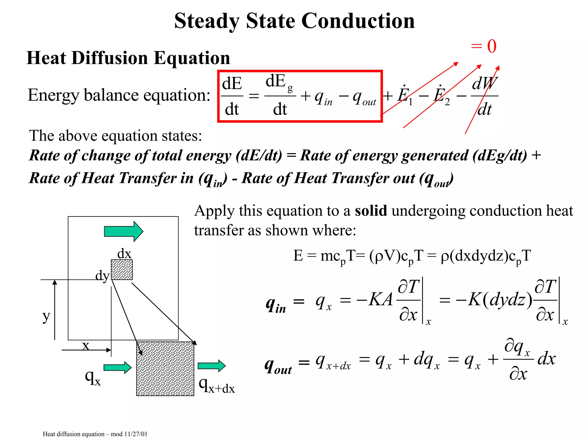
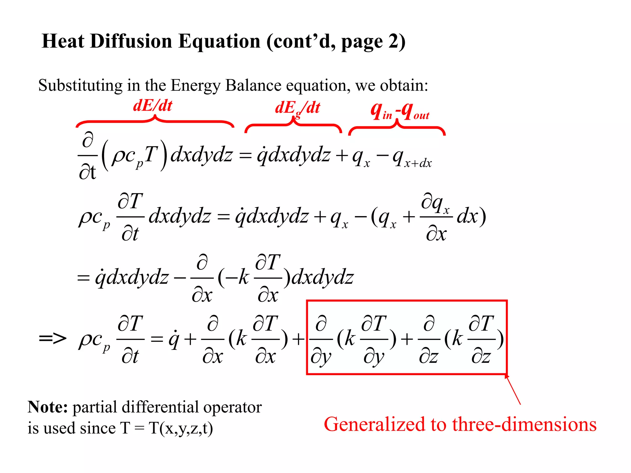
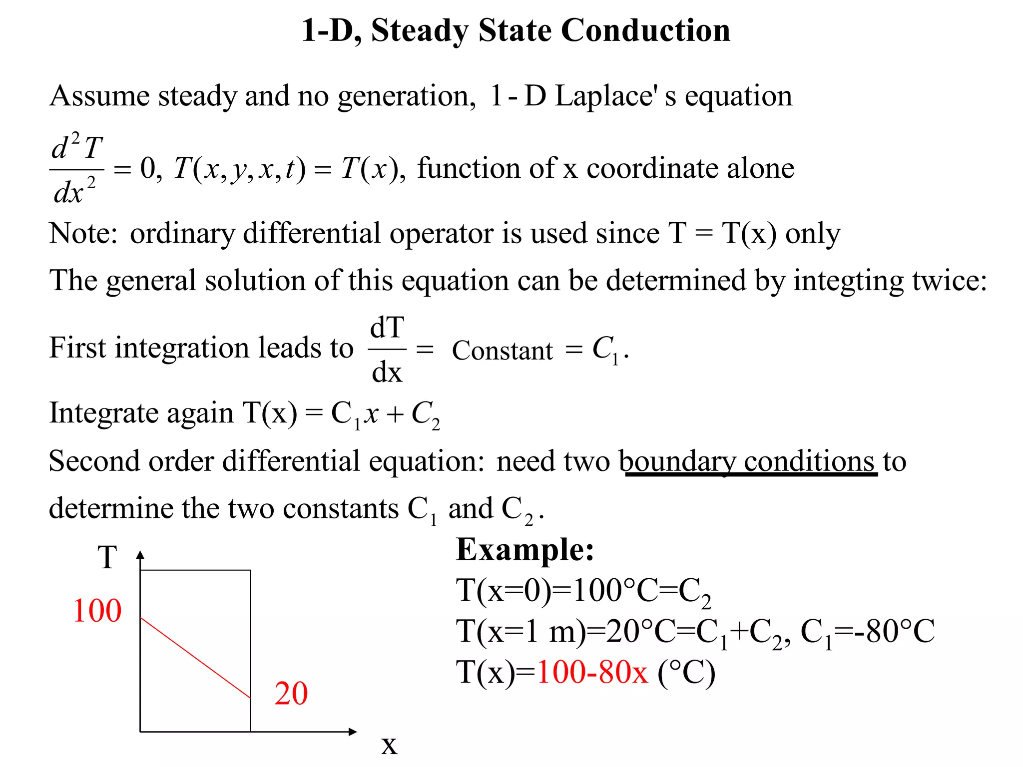
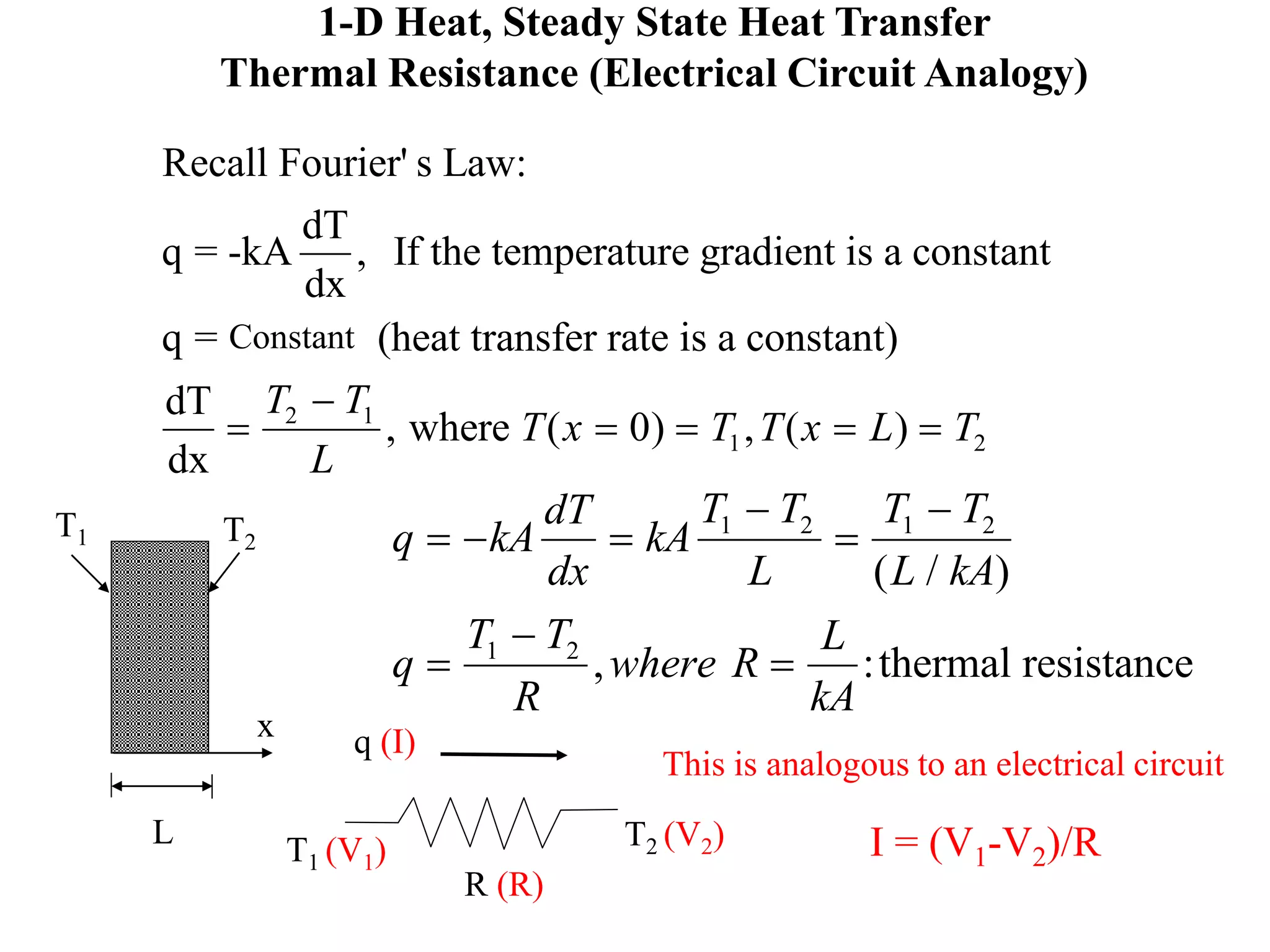
Heat Diffusion Equation
Apply this equation to a solid undergoing conduction heat
transfer as shown where:
E = mcpT= (rV)cpT = r(dxdydz)cpT
Energy balance equation:
dE
dt
dE
dt
g
     
q q E E
dW
dt
in out
 
1 2
x
qx qx+dx
q KA
T
x
K dydz
T
x
q q dq q
q
x
dx
x
x x
x dx x x x
x
 


 


   



( )
= 0
Heat diffusion equation – mod 11/27/01
dy
dx
y
Steady State Conduction
The above equation states:
Rate of change of total energy (dE/dt) = Rate of energy generated (dEg/dt) +
Rate of Heat Transfer in (qin) - Rate of Heat Transfer out (qout)
qin =
qout =
Heat Diffusion Equation (cont’d, page 2)
Generalized to three-dimensions
Note: partial differential operator
is used since T = T(x,y,z,t)
Substituting in the Energy Balance equation, we obtain:
 
Energy Storage = Energy Generation + Net Heat Transfer
t
( )
( )
( ) ( ) ( )
p x x dx
x
p x x
p
c T dxdydz qdxdydz q q
q
T
c dxdydz qdxdydz q q dx
t x
T
qdxdydz k dxdydz
x x
T T T T
c q k k k
t x x y y z z
r
r
r


  



   
 
 
  
 
      
   
      
dE/dt dEg/dt qin -qout
=>
r
r
c
T
t
q
x
k
T
x y
k
T
y z
k
T
z
c
T
t
k
T
x
T
y
T
z
q k T q
where
x y z
T
T
x
T
y
T
z
p
p


 

























   
 











 









 ( ) ( ) ( )

( )  ,

,
Special case1: no generation q = 0
Special case 2: constant thermal conductivity k = constant
is the Laplacian operator
Special case 3:
t
and q = 0
The famous Laplace'
2
2
2
2
2
2
2
2
2
2
2
2
2
2
2
2
2
2
2
2
2
0
0 s equation
Heat Diffusion Equation (cont’d, page 3)
1-D, Steady State Conduction
Assume steady and no generation, 1- D Laplace' s equation
function of x coordinate alone
Note: ordinary differential operator is used since T = T(x) only
The general solution of this equation can be determined by integting twice:
First integration leads to
dT
dx
Integrate again T(x) = C
Second order differential equation: need two boundary conditions to
determine the two constants C and C
1
1 2
d T
dx
T x y x t T x
cons t C
x C
2
2
1
2
0
 
 

, ( , , , ) ( ),
tan .
.
Example:
T(x=0)=100°C=C2
T(x=1 m)=20°C=C1+C2, C1=-80°C
T(x)=100-80x (°C)
100
20
T
x
Constant
1-D Heat, Steady State Heat Transfer
Thermal Resistance (Electrical Circuit Analogy)
Recall Fourier' s Law:
q = -kA
dT
dx
If the temperature gradient is a constant
q = constent (heat transfer rate is a constant)
dT
dx
where
,
, ( ) , ( )


   
T T
L
T x T T x L T
2 1
1 2
0
T1 T2
x
L
q kA
dT
dx
kA
T T
L
T T
L kA
q
T T
R
where R
L
kA
  






1 2 1 2
1 2
( / )
, :thermal resistance
q (I)
T1 (V1) T2 (V2)
R (R)
This is analogous to an electrical circuit
I = (V1-V2)/R
Constant
Thermal Resistance - Composite Wall Heat Transfer
T2
T1
R1=L1/(k1A) R2=L2/(k2A)
T
1 2 1 2 1 2
1 2 1 2
1 2
1 1
1 1 1
1 1
T
Also, q= ,
T T T T T T
q
R R R L L
k A k A
T L
T T qR T q
R k A
  
  
    

   
   
 

     
 
T1 T2
L1 L2
k1 k2
T
Use of the thermal resistance concept make the analysis of complex geometries
relatively easy, as discussed in the example below.
However, note that the thermal heat resistance concept can only be applied for
steady state heat transfer with no heat generation.
Example: Consider a composite wall made of two different materials
Composite Wall Heat Transfer (cont’d)
R1=L1/(k1A) R2=L2/(k2A)
T2
T1 T
T1 T2
L1 L2
k1 k2
T
•Now consider the case where we have 2 different fluids on either sides of the wall at
temperatures, T,1 and T,2 , respectively.
• There is heat transfer by convection from the first fluid (on left) to material 1
and from material 2 to the second fluid (on right).
• Similar to conduction resistance, we can determine the convection resistance,
where Rconv = 1/hA
T,1 T,2
T,1
T,2
Rconv,1= 1/(h1A)
Rconv,2= 1/(h2A)
1
1
1
,
1
2
, 2
,
2
,
R
T
T
R
T
T
R
T
T
Q
conv
tot





 
 

where
2
,
2
,
2
2 2
conv
R
T
T
R
T
T 




This approach can be extended to much more complex geometries
(see YAC, 8-4 and 8-5)
“R” value of insulations
Q: Why is the Rvalue given by L/k ?
A: From previous slide, we know that the thermal resistance to conduction is
defined as the temperature difference across the insulation by the heat flux going
through it, hence:
R
T
q
T
k T
x
x
k
  
 



"
Example:
The typical space inside the residential frame wall is 3.5 in. Find the R-value if
the wall cavity is filled with fiberglass batt. (k=0.046 W/m.K=0.027 Btu/h.ft.R)
R
x
k
ft
Btu h ft R
R ft h Btu R
    
 0 292
0 027
10 8 11
2
.
. / . .
. ( . . / )
In the US, insulation materials are often specified in terms of their thermal
resistance, denoted as R values, where Rvalue = L/k (thickness/thermal conductivity)
In the US, it has units of (hr ft2 °F)/Btu (Note: 1 Btu=1055 J)
R-11 for wall, R-19 to R-31 for ceiling.

heat diffusion equation.ppt

  • 1.
    Heat Diffusion Equation Applythis equation to a solid undergoing conduction heat transfer as shown where: E = mcpT= (rV)cpT = r(dxdydz)cpT Energy balance equation: dE dt dE dt g       q q E E dW dt in out   1 2 x qx qx+dx q KA T x K dydz T x q q dq q q x dx x x x x dx x x x x                ( ) = 0 Heat diffusion equation – mod 11/27/01 dy dx y Steady State Conduction The above equation states: Rate of change of total energy (dE/dt) = Rate of energy generated (dEg/dt) + Rate of Heat Transfer in (qin) - Rate of Heat Transfer out (qout) qin = qout =
  • 2.
    Heat Diffusion Equation(cont’d, page 2) Generalized to three-dimensions Note: partial differential operator is used since T = T(x,y,z,t) Substituting in the Energy Balance equation, we obtain:   Energy Storage = Energy Generation + Net Heat Transfer t ( ) ( ) ( ) ( ) ( ) p x x dx x p x x p c T dxdydz qdxdydz q q q T c dxdydz qdxdydz q q dx t x T qdxdydz k dxdydz x x T T T T c q k k k t x x y y z z r r r                                        dE/dt dEg/dt qin -qout =>
  • 3.
    r r c T t q x k T x y k T y z k T z c T t k T x T y T z qk T q where x y z T T x T y T z p p                                                           ( ) ( ) ( )  ( )  ,  , Special case1: no generation q = 0 Special case 2: constant thermal conductivity k = constant is the Laplacian operator Special case 3: t and q = 0 The famous Laplace' 2 2 2 2 2 2 2 2 2 2 2 2 2 2 2 2 2 2 2 2 2 0 0 s equation Heat Diffusion Equation (cont’d, page 3)
  • 4.
    1-D, Steady StateConduction Assume steady and no generation, 1- D Laplace' s equation function of x coordinate alone Note: ordinary differential operator is used since T = T(x) only The general solution of this equation can be determined by integting twice: First integration leads to dT dx Integrate again T(x) = C Second order differential equation: need two boundary conditions to determine the two constants C and C 1 1 2 d T dx T x y x t T x cons t C x C 2 2 1 2 0      , ( , , , ) ( ), tan . . Example: T(x=0)=100°C=C2 T(x=1 m)=20°C=C1+C2, C1=-80°C T(x)=100-80x (°C) 100 20 T x Constant
  • 5.
    1-D Heat, SteadyState Heat Transfer Thermal Resistance (Electrical Circuit Analogy) Recall Fourier' s Law: q = -kA dT dx If the temperature gradient is a constant q = constent (heat transfer rate is a constant) dT dx where , , ( ) , ( )       T T L T x T T x L T 2 1 1 2 0 T1 T2 x L q kA dT dx kA T T L T T L kA q T T R where R L kA          1 2 1 2 1 2 ( / ) , :thermal resistance q (I) T1 (V1) T2 (V2) R (R) This is analogous to an electrical circuit I = (V1-V2)/R Constant
  • 6.
    Thermal Resistance -Composite Wall Heat Transfer T2 T1 R1=L1/(k1A) R2=L2/(k2A) T 1 2 1 2 1 2 1 2 1 2 1 2 1 1 1 1 1 1 1 T Also, q= , T T T T T T q R R R L L k A k A T L T T qR T q R k A                                T1 T2 L1 L2 k1 k2 T Use of the thermal resistance concept make the analysis of complex geometries relatively easy, as discussed in the example below. However, note that the thermal heat resistance concept can only be applied for steady state heat transfer with no heat generation. Example: Consider a composite wall made of two different materials
  • 7.
    Composite Wall HeatTransfer (cont’d) R1=L1/(k1A) R2=L2/(k2A) T2 T1 T T1 T2 L1 L2 k1 k2 T •Now consider the case where we have 2 different fluids on either sides of the wall at temperatures, T,1 and T,2 , respectively. • There is heat transfer by convection from the first fluid (on left) to material 1 and from material 2 to the second fluid (on right). • Similar to conduction resistance, we can determine the convection resistance, where Rconv = 1/hA T,1 T,2 T,1 T,2 Rconv,1= 1/(h1A) Rconv,2= 1/(h2A) 1 1 1 , 1 2 , 2 , 2 , R T T R T T R T T Q conv tot           where 2 , 2 , 2 2 2 conv R T T R T T      This approach can be extended to much more complex geometries (see YAC, 8-4 and 8-5)
  • 8.
    “R” value ofinsulations Q: Why is the Rvalue given by L/k ? A: From previous slide, we know that the thermal resistance to conduction is defined as the temperature difference across the insulation by the heat flux going through it, hence: R T q T k T x x k         " Example: The typical space inside the residential frame wall is 3.5 in. Find the R-value if the wall cavity is filled with fiberglass batt. (k=0.046 W/m.K=0.027 Btu/h.ft.R) R x k ft Btu h ft R R ft h Btu R       0 292 0 027 10 8 11 2 . . / . . . ( . . / ) In the US, insulation materials are often specified in terms of their thermal resistance, denoted as R values, where Rvalue = L/k (thickness/thermal conductivity) In the US, it has units of (hr ft2 °F)/Btu (Note: 1 Btu=1055 J) R-11 for wall, R-19 to R-31 for ceiling.