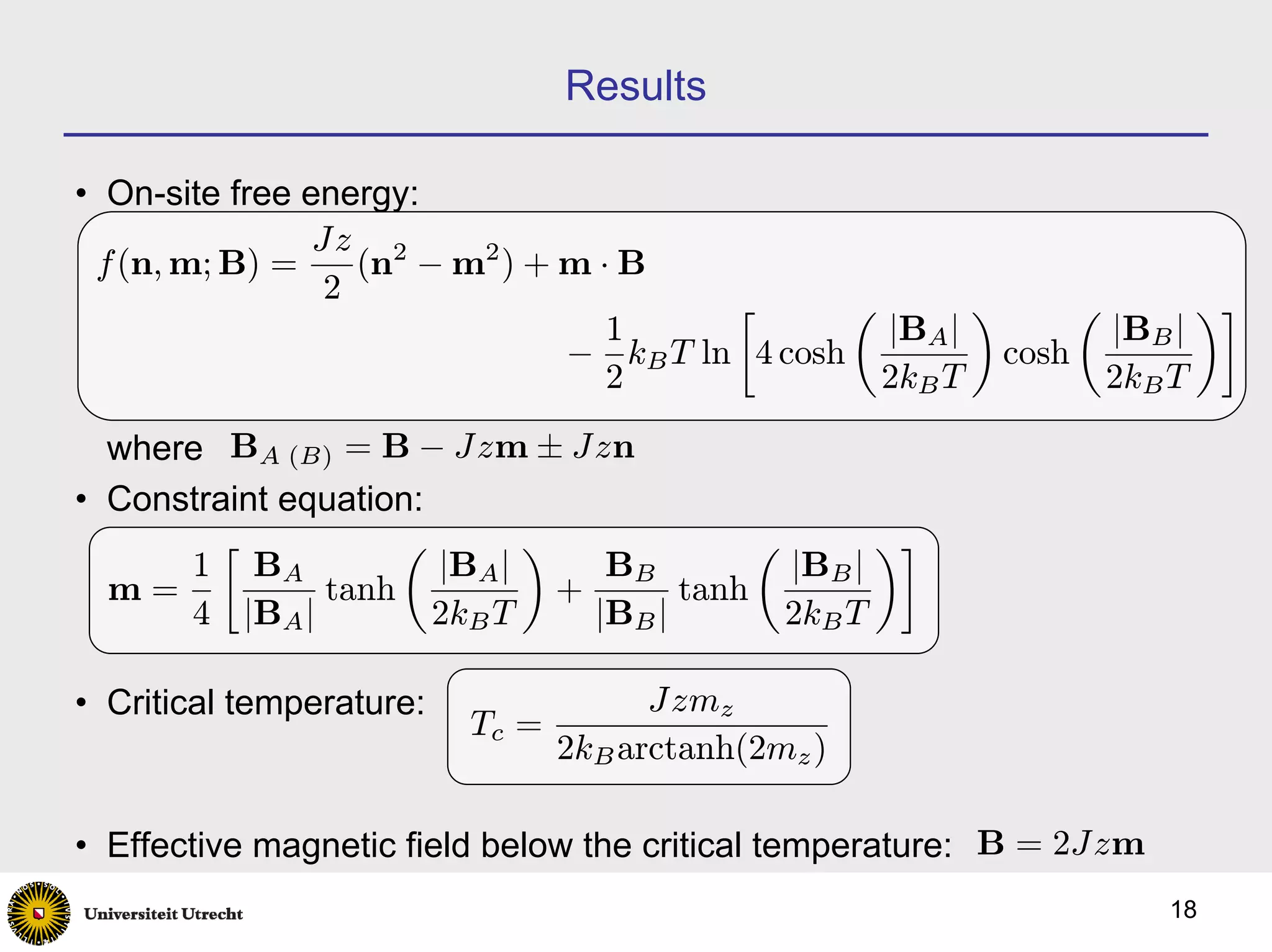
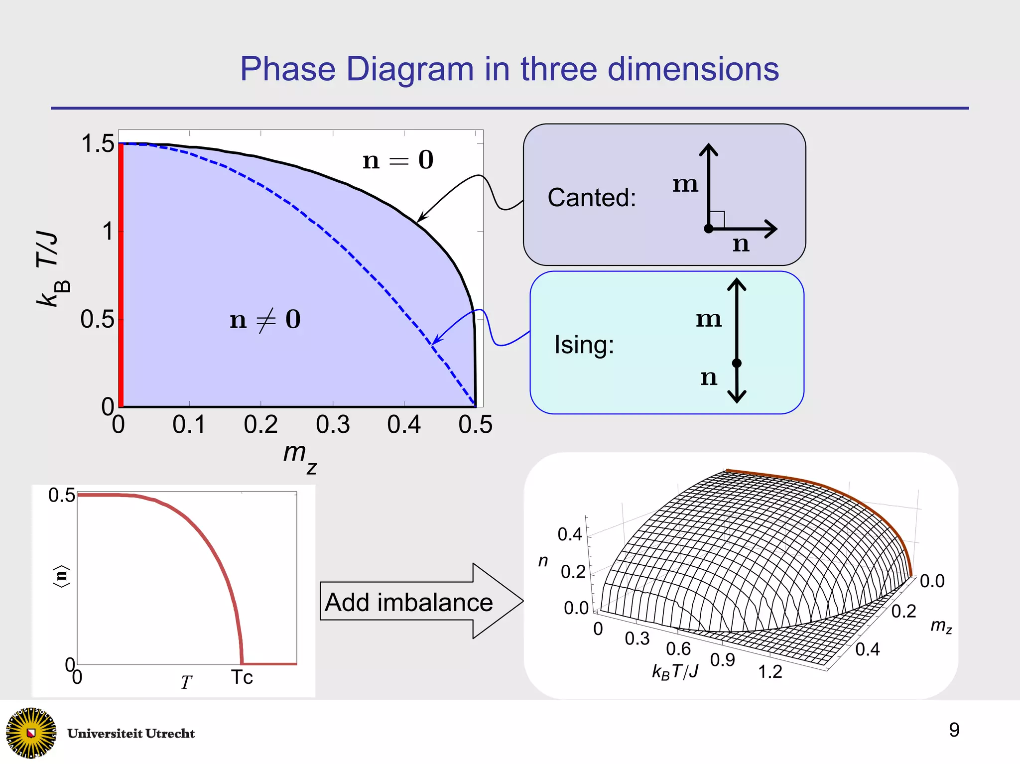
The document summarizes research on the imbalanced antiferromagnet in an optical lattice. Key points: 1) A mean-field analysis of the Fermi-Hubbard model at half filling predicts a Mott insulator phase transition and Néel antiferromagnetic ordering below a critical temperature. 2) Introducing spin imbalance splits the spin-wave dispersion and leads to three phases in the mean-field phase diagram: Néel, canted, and Ising phases. 3) Topological excitations called merons are predicted at low temperatures, whose unbinding drives a Kosterlitz-Thouless transition lowering the critical temperature compared to mean-field theory.

1. The imbalanced antiferromagnet
in an optical lattice
Arnaud Henk Stoof
Koetsier
Floris van Liere

2. Introduction
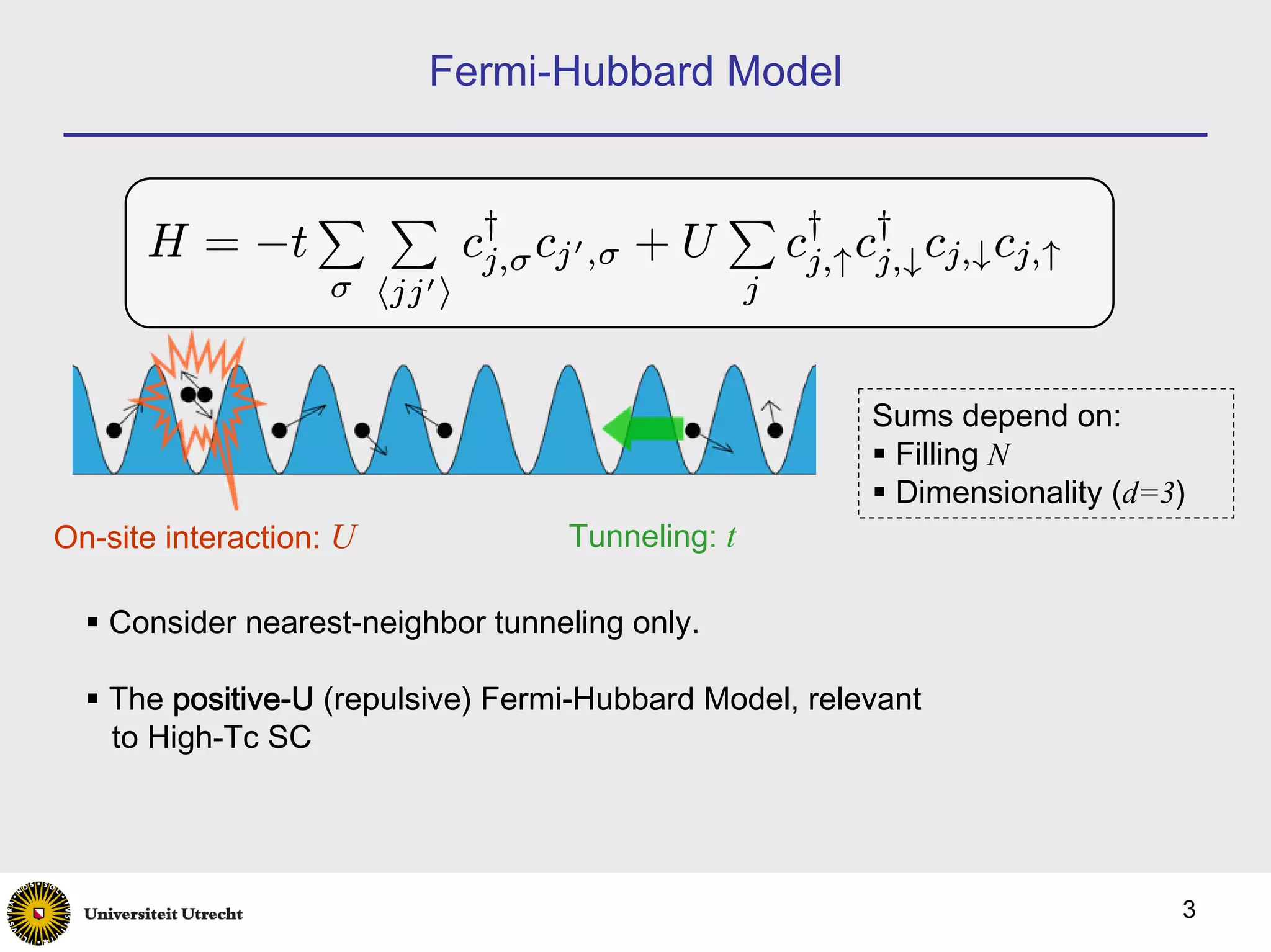
• Fermions in an optical lattice
• Described by the Hubbard model
• Realised experimentally [Esslinger ’05]
• Fermionic Mott insulator recently seen [Esslinger ’08, Bloch
’08]
• There is currently a race to create the Néel state
• Imbalanced Fermi gases
• Experimentally realised [Ketterle ’06, Hulet ’06]
• High relevance to other areas of physics (particle
physics, neutron stars, etc.)
• Imbalanced Fermi gases in an optical lattice ??
2

3. Fermi-Hubbard Model
P P P
H = −t c† cj 0 ,σ
j,σ +U c† c† cj,↓ cj,↑
j,↑ j,↓
σ hjj 0 i j
Sums depend on:
Filling N
Dimensionality (d=3)
On-site interaction: U Tunneling: t
Consider nearest-neighbor tunneling only.
The positive-U (repulsive) Fermi-Hubbard Model, relevant
to High-Tc SC
3

4. Quantum Phases of the Fermi-Hubbard Model
• Positive U (repulsive on-site interaction):
Conductor
1
Filling Fraction
Band Insulator
Conductor
0.5
Conductor Mott Insulator (need large U)
0
• Negative U: Pairing occurs — BEC/BCS superfluid at all fillings.
4

5. Mott insulator: Heisenberg Model (no imbalance yet)
• At half filling, when U À t and kB T ¿ U we are deep in the Mott phase.
Hopping is energetically supressed
Model simplifies: only spin degrees of freedom remain (no transport)
• Integrate out the hopping fluctuations, then the Hubbard model reduces to the
Heisenberg model:
J X
H= S j · Sk
2
hjki
Spin ½ operators: S = 1 σ z 1³ † †
´
2 Si = ci,↑ ci,↑ − ci,↓ ci,↓
2
Si =c† ci,↓
+
i,↑
Si =c† ci,↑
−
i,↓
4t2
Superexchange constant (virtual hops): J=
U
5

6. Néel State (no imbalance yet)
• The Néel state is the antiferromagnetic ground state for J > 0
• Néel order parameter 0 ≤ h|n|i ≤ 0.5
measures amount of “anti-alignment”: 0.5
nj = (−1)j hSj i
〈n〉
h|n|i
• Below some critical temperature Tc,
we enter the Néel state and h|n|i
becomes non-zero.
0
0 T Tc
6

7. Heisenberg Model with imbalance
• Until now, N↑ = N↓ = N/2
• Now take N↑ 6= N↓ — spin population imbalance.
• This gives rise to an overal magnetization m = (0, 0, mz )
N↑ − N↓ (fermions: S = 1 )
mz = S 2
N↑ + N↓
• Add a constraint to the Heisenberg model that enforces hSi = m
J X X
H= S j · Sk − B · (Si − m)
2
hjki i
Effective magnetic field (Lagrange multiplier): B
7

8. Mean field analysis
• J > 0 ⇒ ground state is antiferromagnetic (Néel state)
Two sublattices: A, B
A(B) A(B) A(B)
• Linearize Hamiltonian: Si = hSi i + δSi
B A B
hSA i + hSB i
• Magnetization: m= A B A
2
B A B
A B
hS i − hS i
• Néel order parameter: n=
2 A B A
• Obtain the on-site free energy f (n, m; B)
subject to the constraint ∇B f = 0 (eliminates B)
8

9. Phase Diagram in three dimensions
1.5
n=0
m
Canted:
1 n
kB T/J
0.5 n 6= 0 m
Ising:
n
0
0 0.1 0.2 0.3 0.4 0.5
mz
0.5
0.4
n
〈n〉
0.2
0.0
Add imbalance 0.0 0.2
0 mz
0.3
0.6 0.4
0 0.9
0 Tc kB T J 1.2
T
9

10. Spin waves (magnons)
dS i
• Spin dynamics can be found from: = [H, S]
dt ~
No imbalance: Doubly 0.5
degenerate antiferromagnetic
dispersion
0.4
• Imbalance splits the
¯ ω/J z
0.3
degeneracy:
0.2 Gap:
h
Ferromagnetic (Larmor
magnons: ω ∝ k2 0.1 precession
of n)
0 π π
Antiferromagnetic
− 0
magnons: ω ∝ |k| 2 kd 2
10

11. Long-wavelength dynamics: NLσM
• Dynamics are summarised a non-linear sigma model with an action
Z Z ½ µ ¶2
dx 1 ∂n(x, t)
S[n(x, t)] = dt ~ − 2Jzm × n(x, t)
dD 4Jzn2 ∂t
2
¾
Jd
− [∇n(x, t)]2
• lattice spacing: d = λ/2 2
• number of nearest neighbours: z = 2D
• local staggered magnetization: n(x, t)
• The equilibrium value of n(x, t) is found from the Landau free energy:
Z ½ 2 ¾
dx Jd 2
F [n(x), m] = [∇n(x)] + f [n(x), m]
dD 2
• NLσM admits spin waves but also topologically stable excitations in
the local staggered magnetisation n(x, t).
11

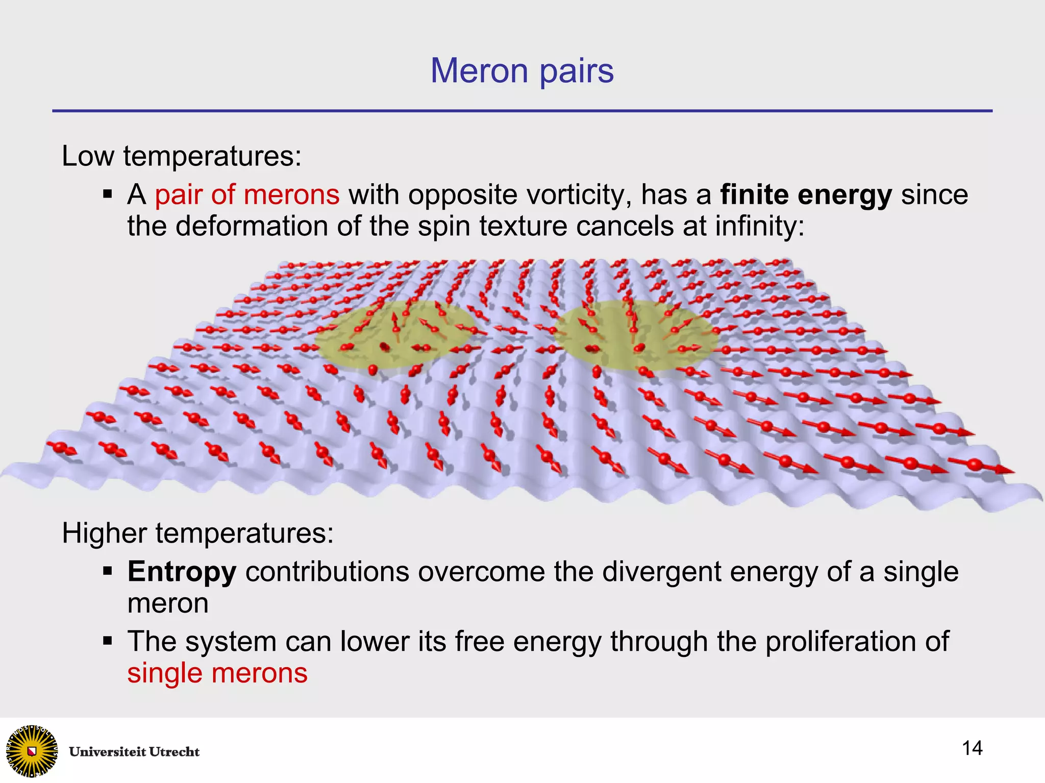
12. Topological excitations
• The topological excitaitons are vortices; Néel vector has an out-of-
easy-plane component in the core
• In two dimensions, these are merons:
• Spin texture of a meron:
⎛ p ⎞
n 2 − [n (r)]2 cos φ
p z
n = ⎝nv n2 − [nz (r)]2 sin φ⎠
nz (r) nv = 1
n
• Ansatz: nz (r) =
[(r/λ)2 + 1]2
• Merons characterised by:
Pontryagin index ±½
Vorticity nv = ±1
Core size λ nv = −1
12

13. Meron size
• Core size λ of meron found by plugging the spin texture into F [n(x), m]
and minimizing (below Tc):
1.5 Meron core size
6
1 Λ
kB T/J
Merons 4
d 2
0.5 present 1.5
1.2
0 0.9
0 0 kB T J
0 0.1 0.2 0.3 0.4 0.5 0.1 0.6
mz 0.2
0.3 0.3
mz 0.4
• The energy of a single meron diverges logarithmically with the
system area A at low temperature as
Jn2 π A
ln 2
2 πλ
merons must be created in pairs.
13

14. Meron pairs
Low temperatures:
A pair of merons with opposite vorticity, has a finite energy since
the deformation of the spin texture cancels at infinity:
Higher temperatures:
Entropy contributions overcome the divergent energy of a single
meron
The system can lower its free energy through the proliferation of
single merons
14

15. Kosterlitz-Thouless transition
• The unbinding of meron pairs in 2D signals a KT transition. This
drives down Tc compared with MFT:
1 MFT in 2D
0.8 0.06
0.6
kB T/J
kB T/J
0.04
n 6= 0
0.4
KT transition 0.02
0.2
0 0
0 0.05 0.1
0 0.2 0.4
mz
mz
• New Tc obtained by analogy to an anisotropic O(3) model (Monte
Carlo results: [Klomfass et al, Nucl. Phys. B360, 264 (1991)] )
15

16. Experimental feasibility
• Experimental realisation:
Imbalance: drive spin transitions with RF field
Néel state in optical lattice: adiabatic cooling [AK et al. PRA77,
023623 (2008)]
• Observation of Néel state
Correlations in atom shot noise
Bragg reflection (also probes spin waves)
• Observation of KT transition
Interference experiment [Hadzibabic et al. Nature 441, 1118 (2006)]
In situ imaging [Gericke et al. Nat. Phys. 4, 949 (2008); Würtz et al.
arXiv:0903.4837]
16

17. Conclusion
• Tc calculated for entering an antiferromagnetically ordered state in mean field
theory
• Topological excitations give rise to a KT transition in 2D which significantly
lowers Tc compared to MFT.
• The imbalanced antiferrromagnet is a rich system
ferro- and antiferromagnetic properties
contains topological excitations
models quantum magnetism, bilayers, etc.
merons possess an internal Ising degree of freedom associated to
Pontryagin index — possible application to topological quantum
computation
• Future work:
include fluctuations beyond MFT for better accuracy in three dimensions
investigate topological excitations in 3D (vortex rings)
incorporate equilibrium in the NLσM
gradient of n gives rise to a magnetization
17

18. Results
• On-site free energy:
Jz 2
f (n, m; B) = (n − m2 ) + m · B
2 ∙ µ ¶ µ ¶¸
1 |BA | |BB |
− kB T ln 4 cosh cosh
2 2kB T 2kB T
where BA (B) = B − Jzm ± Jzn
• Constraint equation:
∙ µ ¶ µ ¶¸
1 BA |BA | BB |BB |
m= tanh + tanh
4 |BA | 2kB T |BB | 2kB T
• Critical temperature: Jzmz
Tc =
2kB arctanh(2mz )
• Effective magnetic field below the critical temperature: B = 2Jzm
18

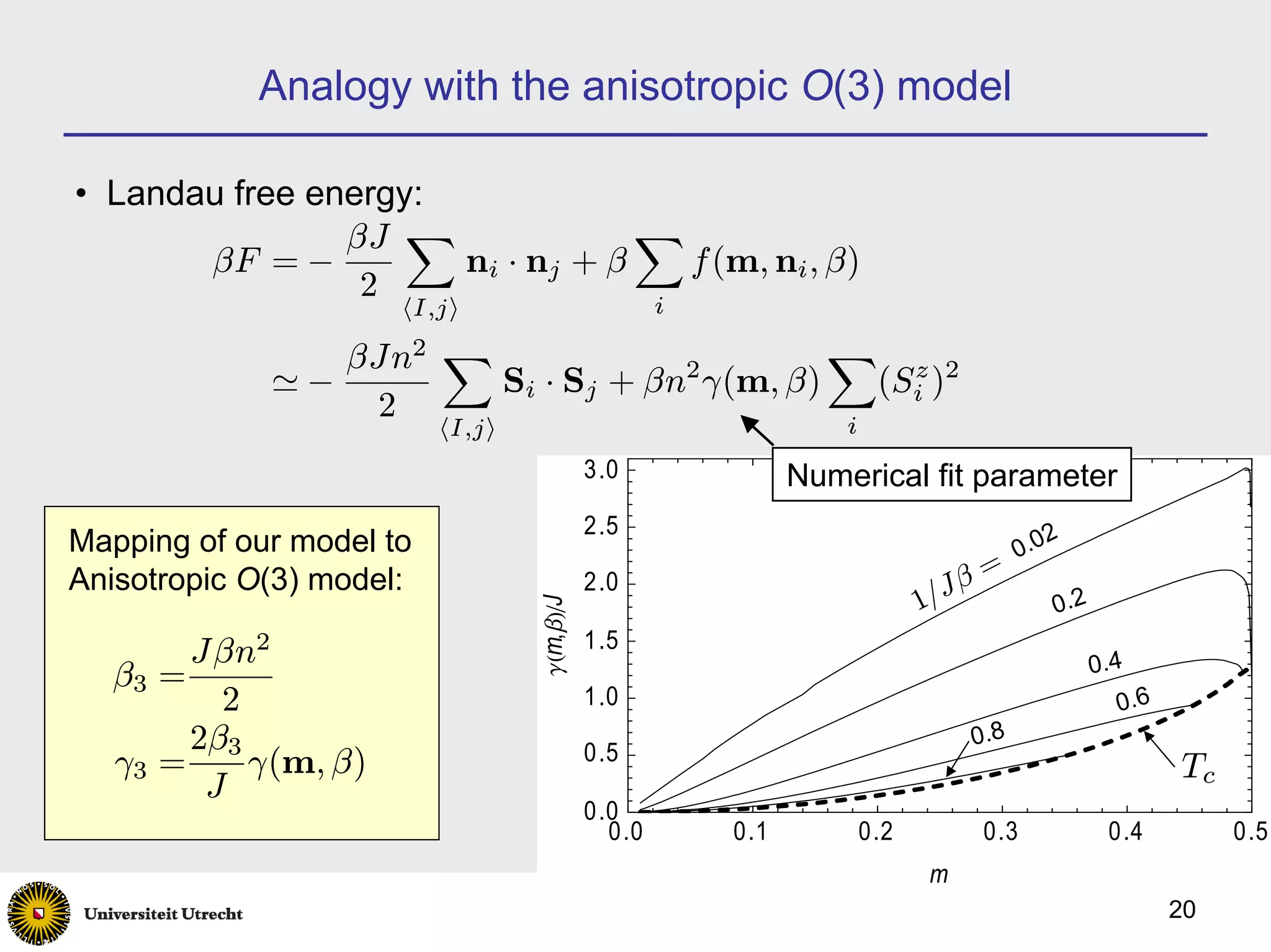
19. Anisotropic O(3) model
• Dimensionless free energy of the anisotropic O(3) model [Klomfass et al, Nucl.
Phys. B360, 264 (1991)] :
X X
βf3 = −β3 Si · Sj + γ3 (Si )2
z
hi,ji i
• KT transition:
1.0
0.8
g3êH1+g3L
0.6
0.4
0.2
0.0
1.0 1.2 1.4 1.6 1.8 2.0
b3
β3
• Numerical fit: γ3 (β3 ) = exp[−5.6(β3 − 1.085)].
β3 − 1.06
19

20. Analogy with the anisotropic O(3) model
• Landau free energy:
βJ X X
βF = − ni · nj + β f (m, ni , β)
2 i
hI,ji
βJn2 X 2
X
'− Si · Sj + βn γ(m, β) (Si )2
z
2 i
hI,ji
3.0 Numerical fit parameter
2.5 2
Mapping of our model to 0.0
Anisotropic O(3) model: 2.0 β =
1/J 0.2
g Hm, bLêJ
1.5
Jβn2 0.4
β3 =
2 1.0 0.6
2β3 0.8
γ3 = γ(m, β) 0.5
Tc
J
0.0
0.0 0.1 0.2 0.3 0.4 0.5
m
20