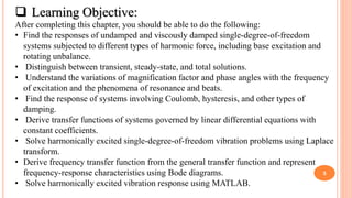
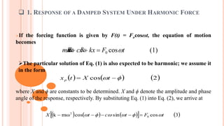
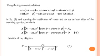
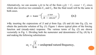
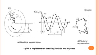
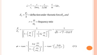
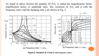
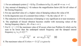
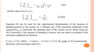
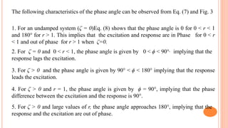
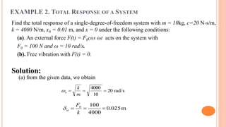
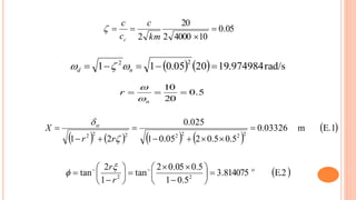
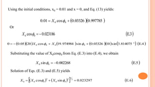
This document provides information about the dynamics of machinery course for several mechanical engineering students. It includes the learning objectives, symbols and definitions, response of a damped system under harmonic motion, an example problem, and key concepts about magnification factor, phase angle, and total response of a system. The example calculates the total response of a single-degree-of-freedom system subjected to an external harmonic force and free vibration.

1. Subject:-Dynamics of Machinery
B.E. Mechanical – Semester 6
(Division-A)

2. MECH. NO: ENROLLMENT
NO:
NAME OF STUDENT:
MECH6051 150150119017 DHAVAL CHAUHAN
MECH6052 150150119067 PRAJESH MARADIYA
MECH6053 160153119009 DHAVAL DARJI
MECH6054 150150119052 SAVAN KARMUR
MECH6055 160153119018 IMARAN MANEK
Prepared by:-

3. PPT OUTLINES
Learning Objective
List of symbol
Response of damped system under harmonic motion
Example (Total response)

4. LIST OF SYMBOL (NOMENCLATURE)
Symbols
Frequency Ratio r
Forcing Frequency ω
Natural Frequency ω 𝑛
Damping Ratio ζ
Frequencies corresponding to half-power
points
ω1, ω2

5. 5
 Learning Objective:
After completing this chapter, you should be able to do the following:
• Find the responses of undamped and viscously damped single-degree-of-freedom
systems subjected to different types of harmonic force, including base excitation and
rotating unbalance.
• Distinguish between transient, steady-state, and total solutions.
• Understand the variations of magnification factor and phase angles with the frequency
of excitation and the phenomena of resonance and beats.
• Find the response of systems involving Coulomb, hysteresis, and other types of
damping.
• Derive transfer functions of systems governed by linear differential equations with
constant coefficients.
• Solve harmonically excited single-degree-of-freedom vibration problems using Laplace
transform.
• Derive frequency transfer function from the general transfer function and represent
frequency-response characteristics using Bode diagrams.
• Solve harmonically excited vibration response using MATLAB.

6.  1. RESPONSE OF A DAMPED SYSTEM UNDER HARMONIC FORCE
If the forcing function is given by F(t) = Focosωt, the equation of motion
becomes
(1)cos0 tFkxxcxm  
     2cos   tXtxp
The particular solution of Eq. (1) is also expected to be harmonic; we assume it
in the form
where X and ϕ are constants to be determined. X and ϕ denote the amplitude and phase
angle of the response, respectively. By substituting Eq. (1) into Eq. (2), we arrive at
        3cossincosmωk 0
2
tFtctX  

7. Using the trigonometric relations
 
  

sincoscossinsin
sinsincoscoscos
ttt
ttt


  
    40coscos
sincos
2
0
2




cmkX
FcmkX
in Eq. (3) and equating the coefficients of cosωt and sin ωt on both sides of the
resulting equation, we obtain
Solution of Eq. (4) gives
  
 5
2
1
2222
0
 cmk
F
X



8. Alternatively, we can assume xp(t) to be of the from xp(t) = C1 cosωt + C2 sinωt,
which also involves two constants C1 and C2. But the final result will be the same in
both cases.
 6tan 2
1







 



mk
c
By inserting the expressions of X and ϕ from Eqs. (5) and (6) into Eq. (2), we
obtain the particular solution of Eq. (1). Figure 1 shows typical plots of the forcing
function and (steady-state) response. The various terms of Eq. (2) are shown
vectorially in Fig. 1. Dividing both the numerator and denominator of Eq. (4) by k
and making the following substitutions
frequency,naturalundapmed
m
k
n

9. Figure 1. Representation of forcing function and response
(a) Graphical representation
(b) Vectorial
representation

10. n
nc mk
c
m
c
c
c


 2
m
c
;
22

and
k
F
st ,Fforcestaticunder thedeflection 0
0

ratiofrequency
n
r


   222
2/1
222
21
1
21
1
rr
X
nn
st








































 7
1
2
tan
1
2
tan 2
1
2
1





























 
r
r
n
n 







11. As stated in above Section the quantity M=X/δst is called the magnification factor,
amplification factor, or amplitude ratio. The variations of X/δst and ϕ with the
frequency ratio r and the damping ratio ζ are shown in Fig. 2.
Figure 2. Variation of X and ϕ with frequency ratio r.
(a) Frequency ratio: r = ω/ωn
(b) Frequency ratio: r = ω/ωn

12. 1. For an undamped system (ζ = 0) Eq. (7) reduces to Eq. (1), and M→∞ as r→1.
2. Any amount of damping (ζ >0) reduces the magnification factor (M) for all values of
the forcing frequency.
3. For any specified value of r, a higher value of damping reduces the value of M.
4. In the degenerate case of a constant force (when r = 0), the value of M = 1.
5. The reduction in M in the presence of damping is very significant at or near resonance.
6. The amplitude of forced vibration becomes smaller with increasing values of the
forcing frequency (that is , M→ 0 as r→∞ ).
7. For 0 < ζ < 1/√2 the maximum value of M occurs when (see Problem 8) which can be
seen to be lower than the undamped natural frequency and the damped natural
frequency wd=wn (1-2ζ2) 1/2.
8. The maximum value of X (when r= √1-2ζ2 ) is given by
 821or21 22
  nr

13.  9
12
1
2
m ax  






st
X
 10
2
1
 






 n
st
x
and the value of X at ω=ωn
Equation (9) can be used for the experimental determination of the measure of
damping present in the system. In a vibration test, if the maximum amplitude of the
response(X)max is measured, the damping ratio of the system can be found using Eq.
(9). Conversely, if the amount of damping is known, one can make an estimate of the
maximum amplitude of vibration.
9. For ζ=1/√2, dM/dr = 0 when r = 0. For ζ>1√1/2, the graph of M monotonically
decreases with increasing values of r.

14. The following characteristics of the phase angle can be observed from Eq. (7) and Fig. 3
1. For an undamped system (ζ = 0)Eq. (8) shows that the phase angle is 0 for 0 < r < 1
and 180° for r > 1. This implies that the excitation and response are in Phase for 0 < r
< 1 and out of phase for r > 1 when ζ=0.
3. For ζ > 0 and the phase angle is given by 90° < ϕ < 180° implying that the response
leads the excitation.
2. For ζ = 0 and 0 < r < 1, the phase angle is given by 0 < ϕ < 90°, implying that the
response lags the excitation.
4. For ζ > 0 and r = 1, the phase angle is given by ϕ = 90°, implying that the phase
difference between the excitation and the response is 90°.
5. For ζ > 0 and large values of r, the phase angle approaches 180°, implying that the
response and the excitation are out of phase.

15. X and ϕ are given by Eqs. (7) and (8), respectively, X0 and ϕ0 [different from those of
Eq. (2)] can be determined from the initial conditions. For the initial conditions
x(t=0)= x0, and x(t=0)=x0 Eq. (11) yields
nd  2
1
 12sinsincos
coscos
00000
000


XXXx
XXx
dn 


       11coscos 00 
 
tXteXtx d
tn
The solution of Eq. (12) gives X0and ϕ0 as
   
 
 13
cos
sincos
tan
sincos
1
cos
0
0
0
2
1
2
002
2
00






Xx
XXxx
XXxxXxX
d
nn
nn
d













16. EXAMPLE 2. TOTAL RESPONSE OF A SYSTEM
Find the total response of a single-degree-of-freedom system with m = 10kg, c=20 N-s/m,
k = 4000 N/m, x0 = 0.01 m, and x = 0 under the following conditions:
(a). An external force F(t) = F0cos ωt acts on the system with
F0 = 100 N and ω = 10 rad/s.
(b). Free vibration with F(t) = 0.
Solution:
(a) from the given data, we obtain
rad/s20
10
4000

m
k
n
m025.0
4000
1000

k
F
st

17. 05.0
1040002
20
2



km
c
c
c
c

    rad/s974984.192005.011
22
 nd 
5.0
20
10

n
r


       
 E.1m03326.0
5.05.0205.01
025.0
21
2222222







rr
X st
 E.2814075.3
5.01
5.005.02
tan
1
2
tan 22
















 
r
r


18. Or
 E.3023186.0cos 00 X
           E.4814075.3sin1003326.0sin974984.19cos2005.00 0000

  XX
      E.6023297.0sincos 2
1
2
00
2
000   XXX
 E.5002268.0sin 00 X
Solution of Eqs. (E.3) and (E.5) yields
Substituting the value of X0cosφ0 from Eq. (E.3) into (E.4), we obtain
  997785.003326.0cos01.0 00  X
Using the initial conditions, x0 = 0.01 and x = 0, and Eq. (13) yields:

19. (B). For free vibration, the total response is given by
 E.7586765.5
or
0978176.0
cos
sin
tan
0
00
00
0







X
X
     E.8cos 00 
 
teXtx d
tn
Using the initial conditions x(0) = x0 = 0.01 of Eq (E.8) can be determined as (see
Eqs. 2.73 and 2.75):
 E.9010012.0
974984.19
01.02005.0
01.0
2
1
2
2
2
1
2
02
0 













 
















d
n x
xX



20.  E.10865984.2
974984.19
2005.0
tantan 1
0
00
0
1
0

 




 





 
 
x
xx
x
d
n



Note that the constant X0 and ϕ0 in case (a) and (b) are very different.