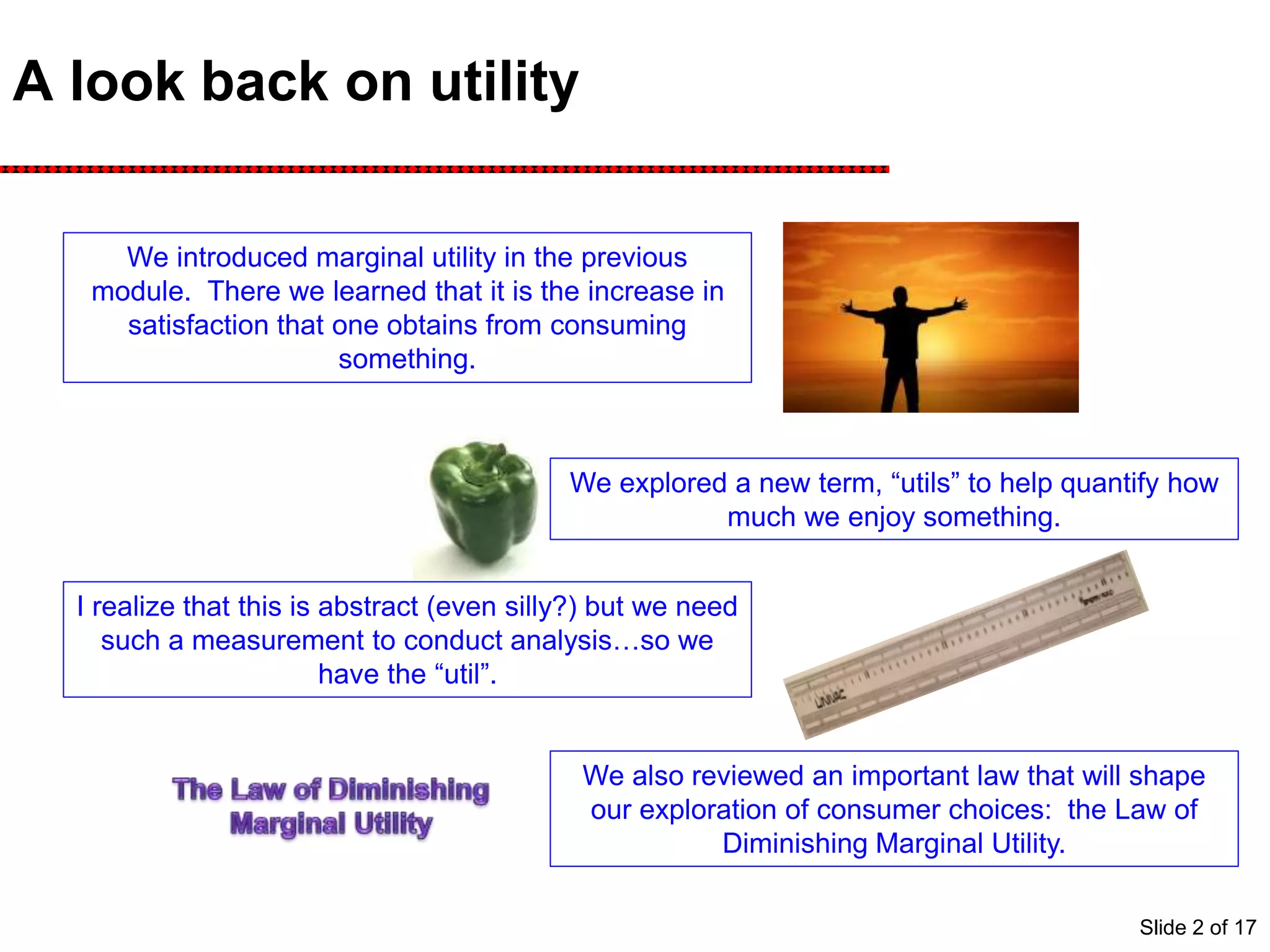
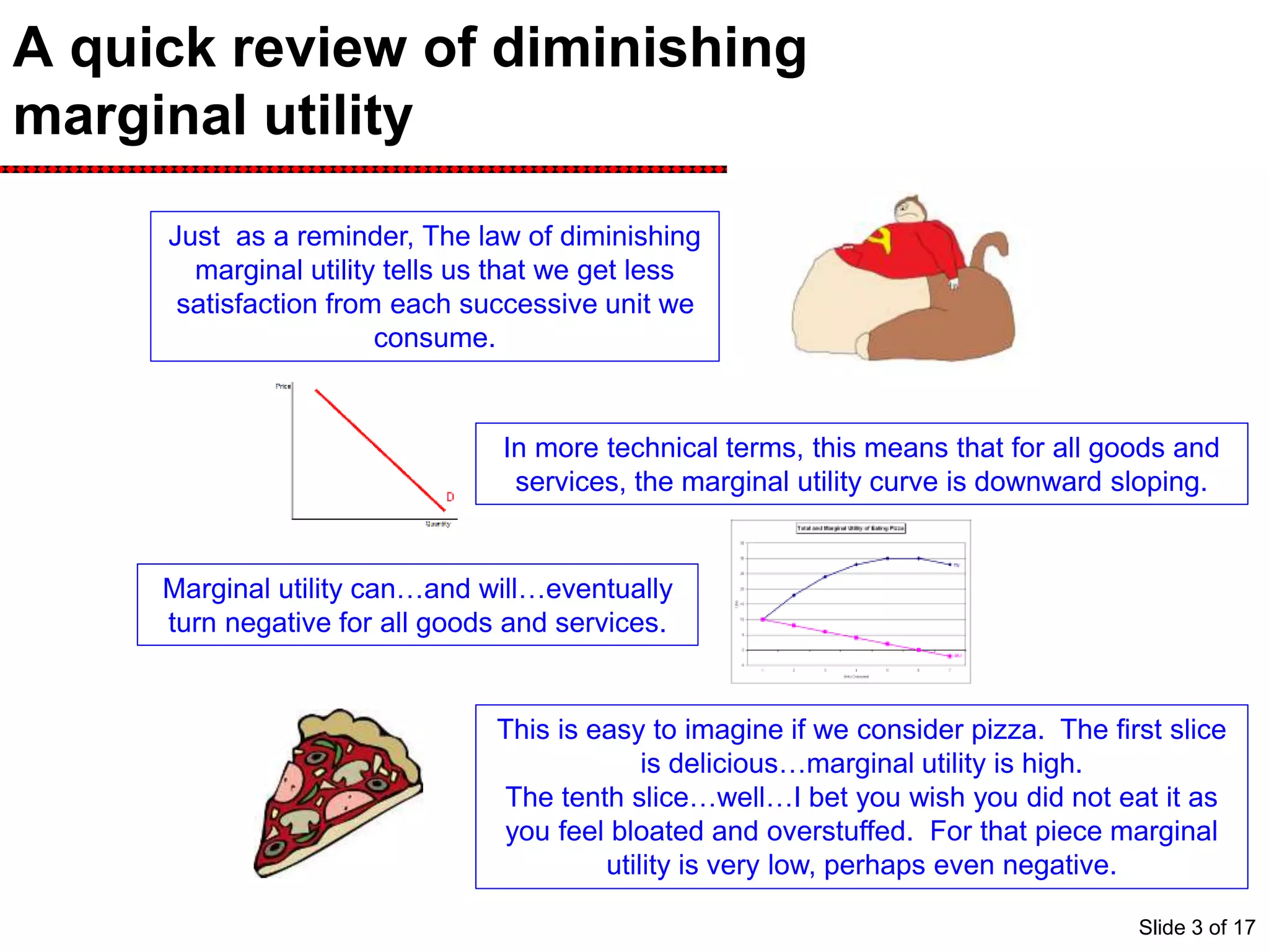
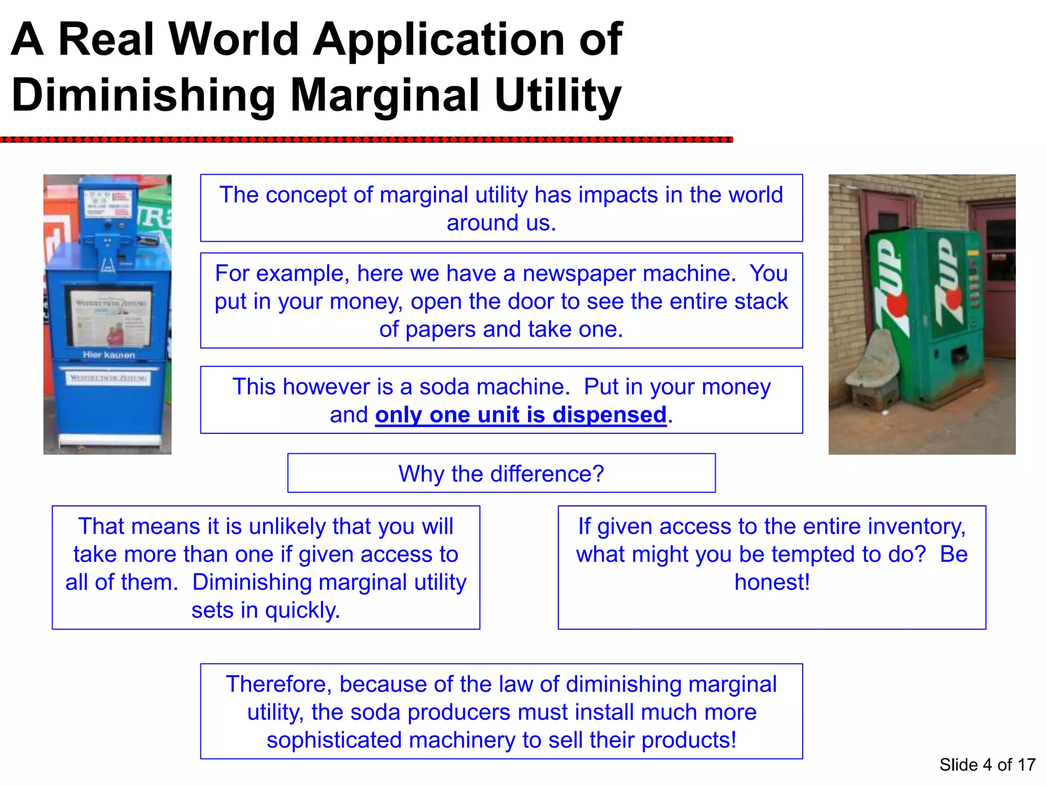
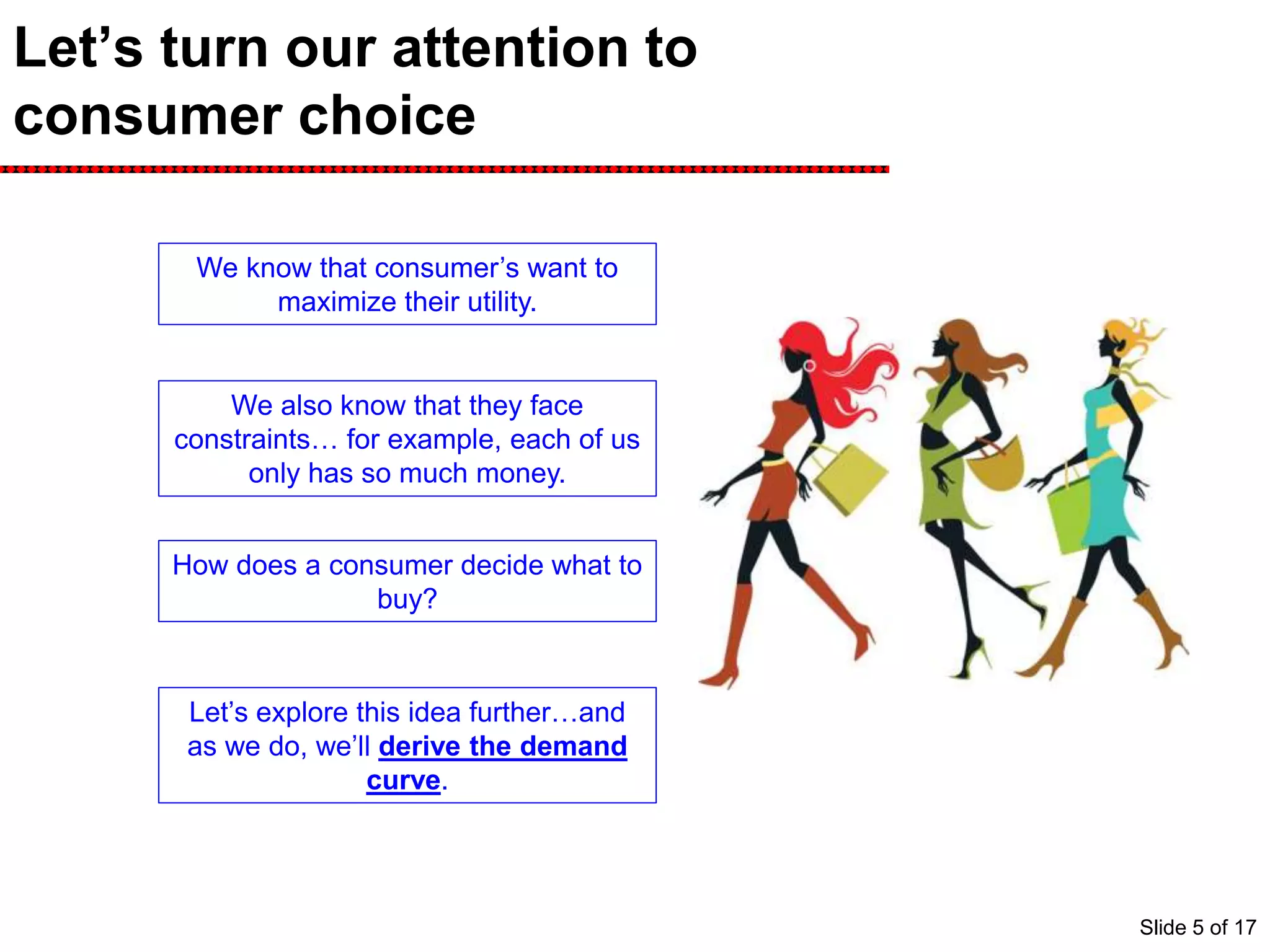
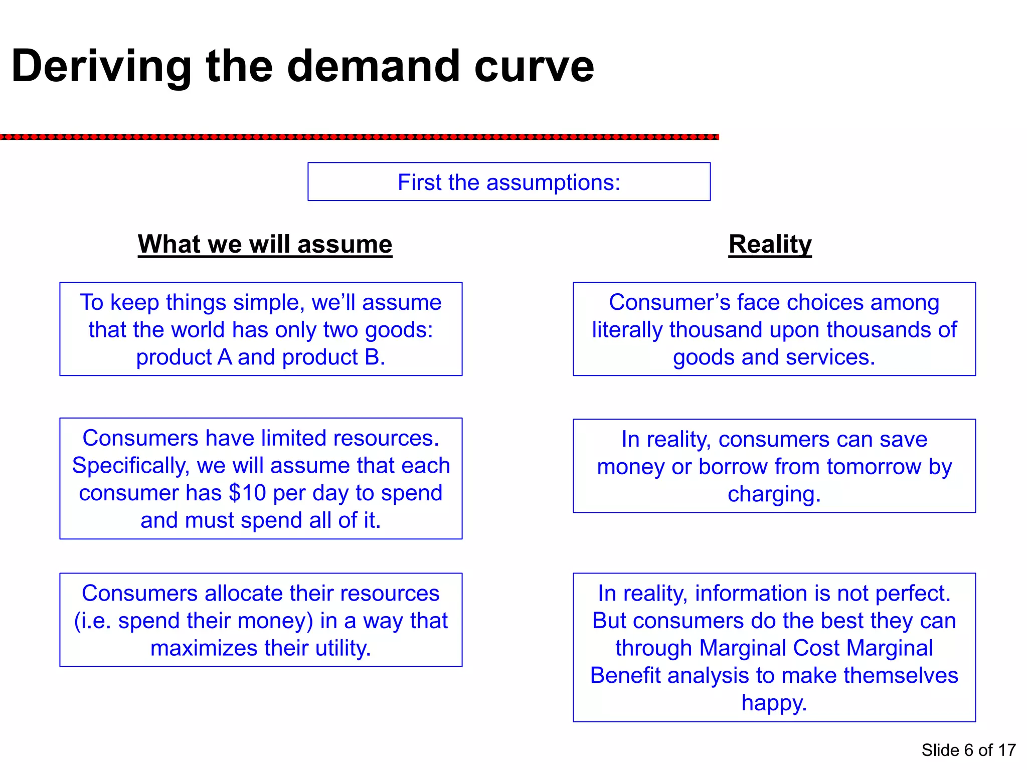
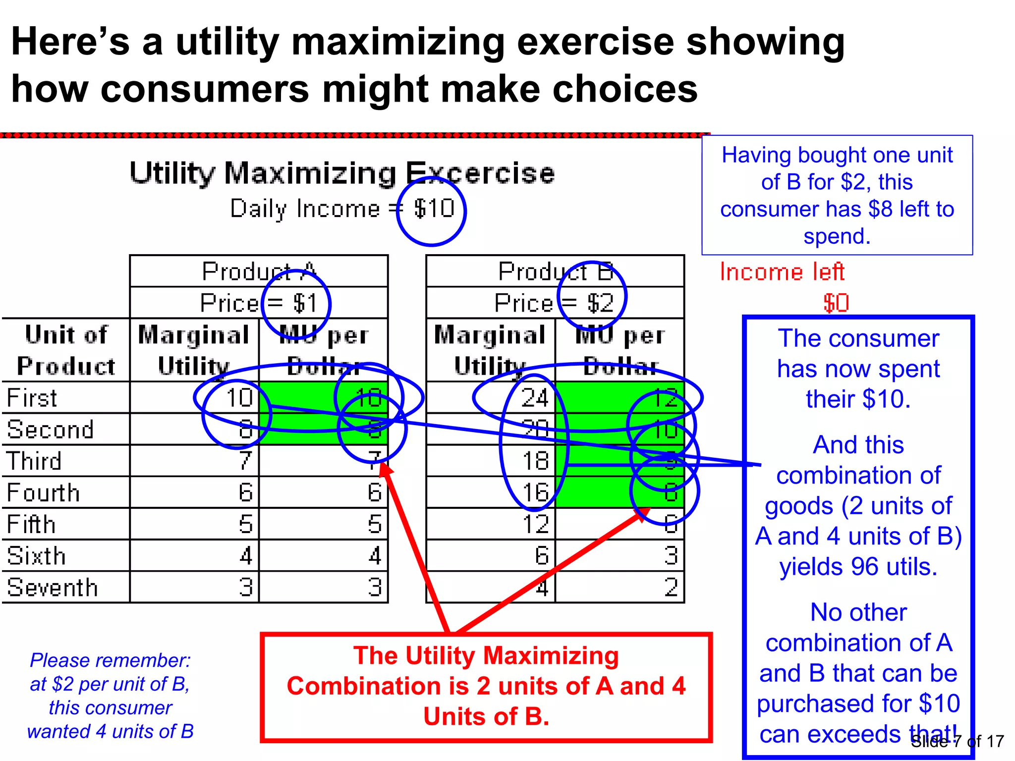
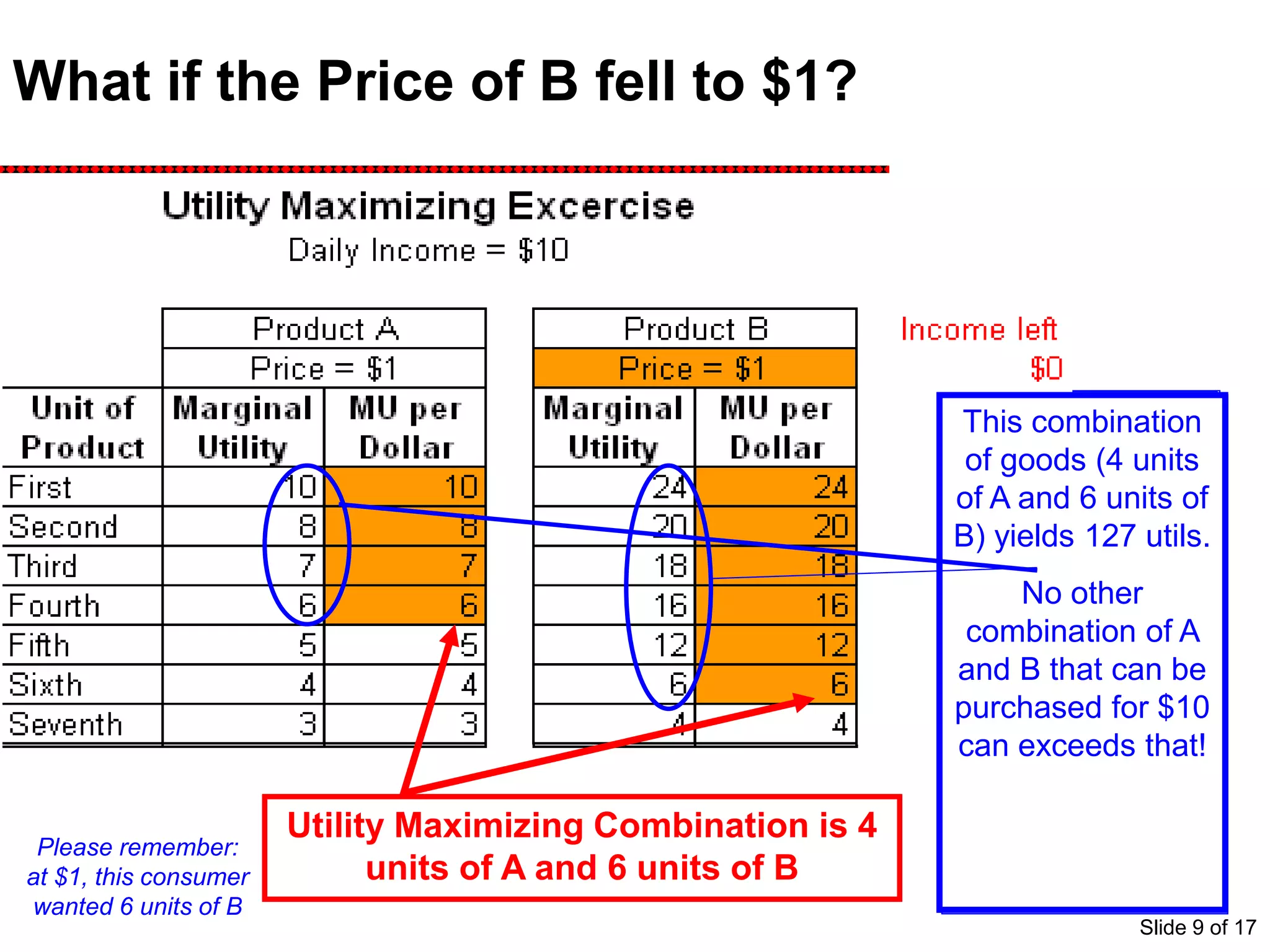
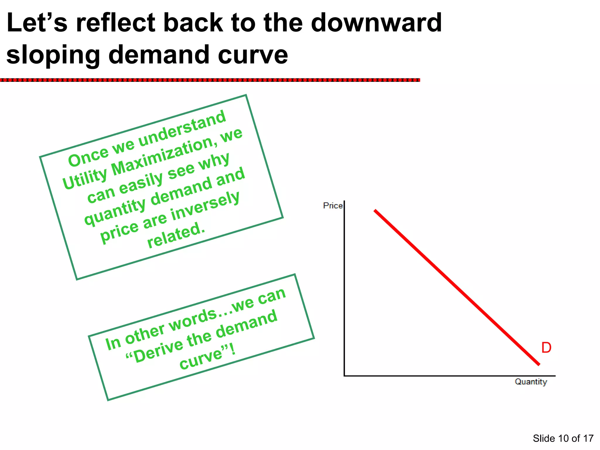
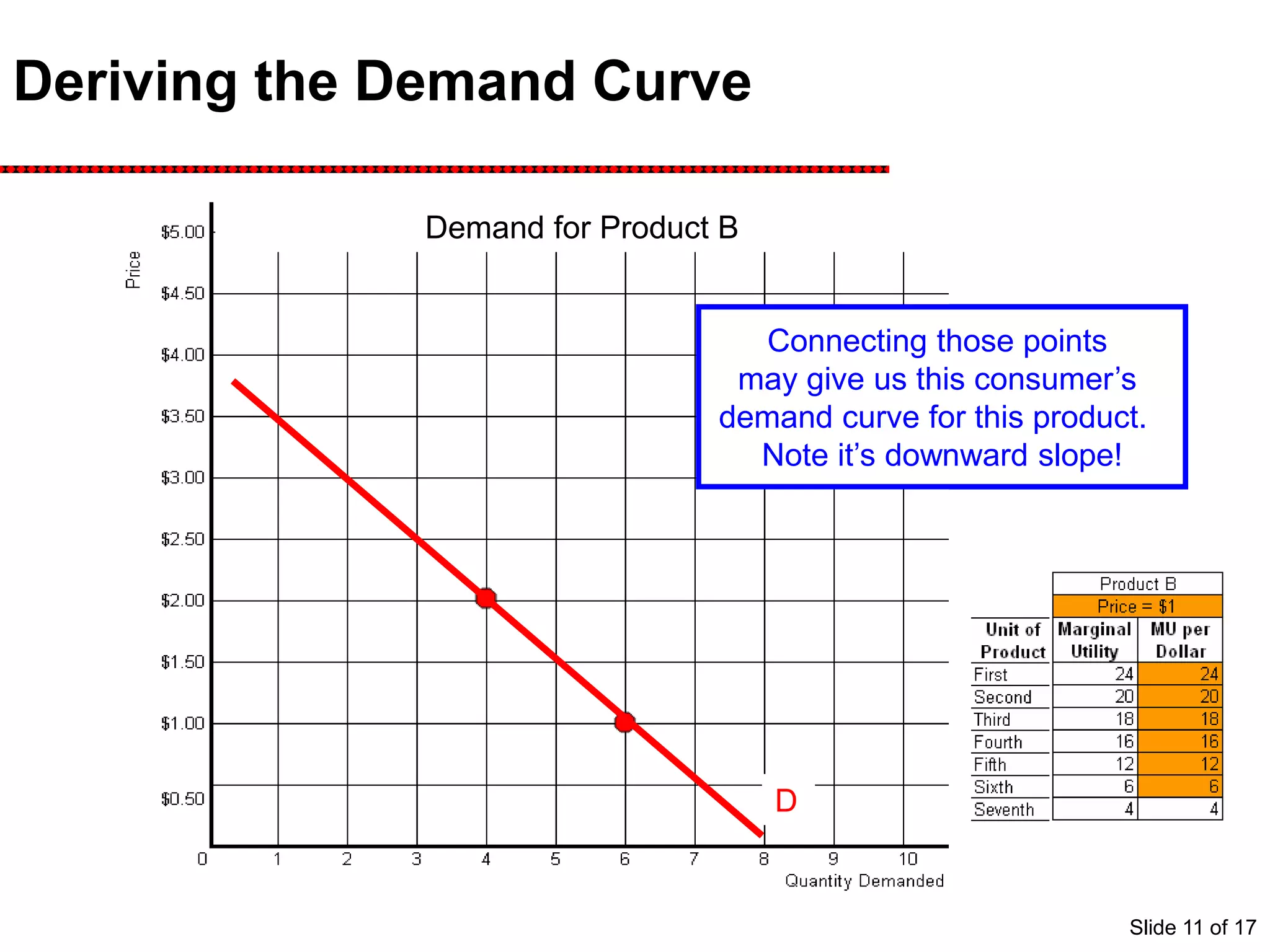
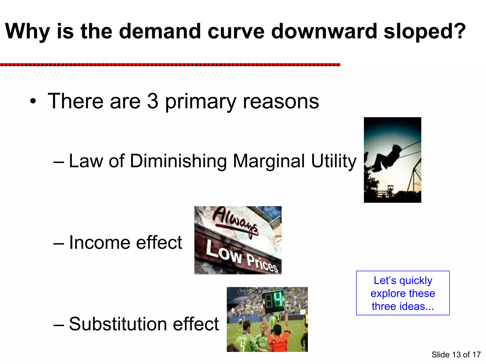
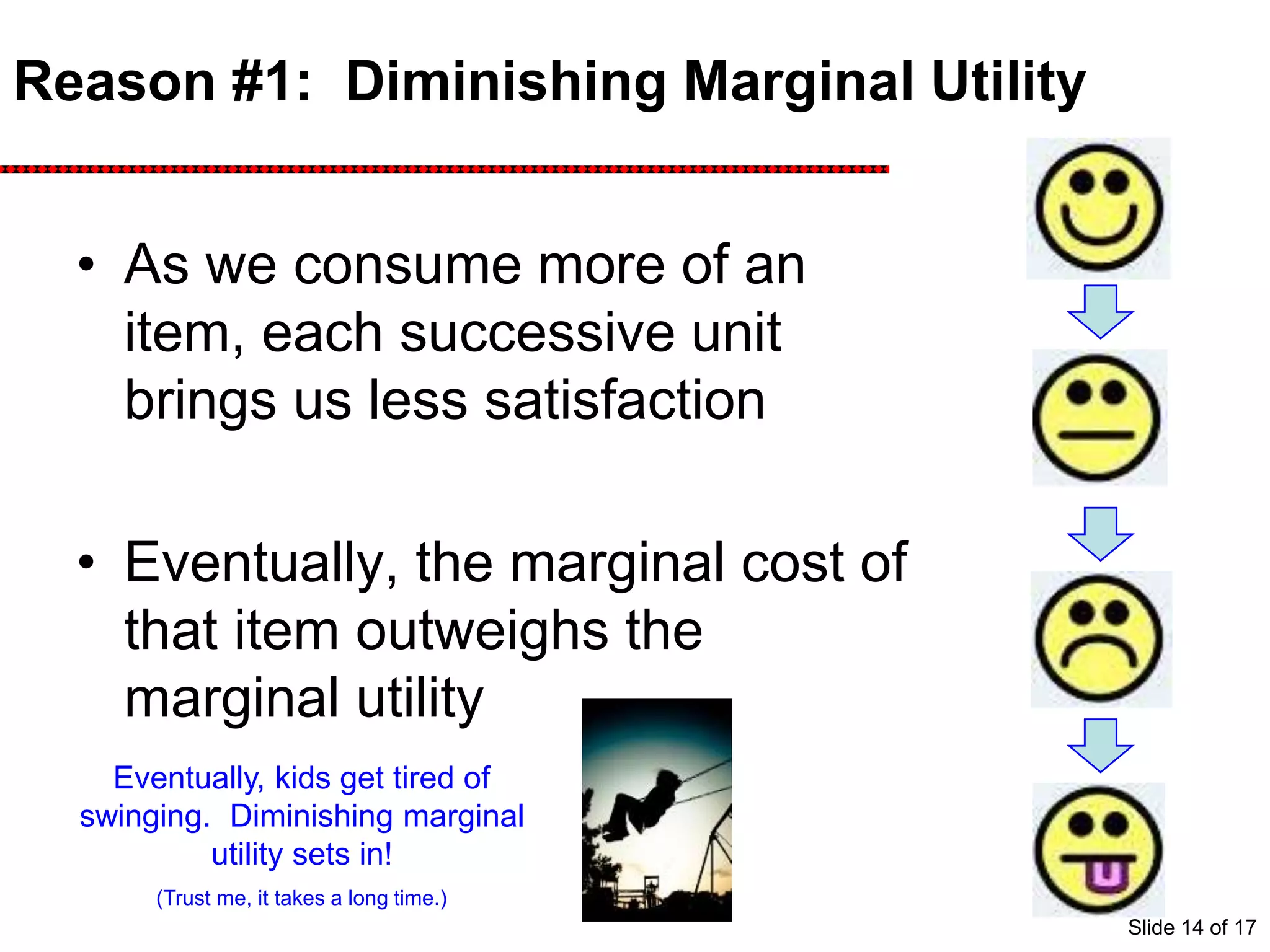
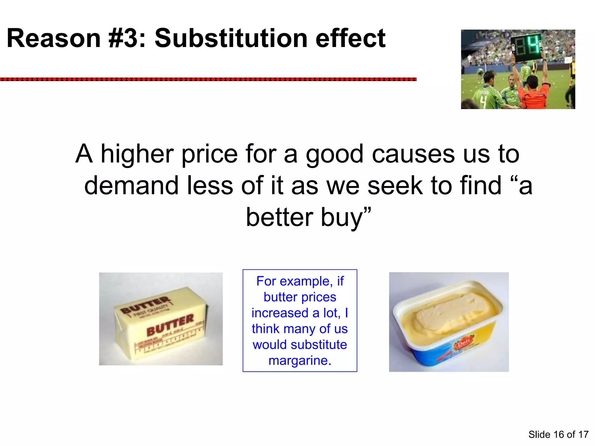
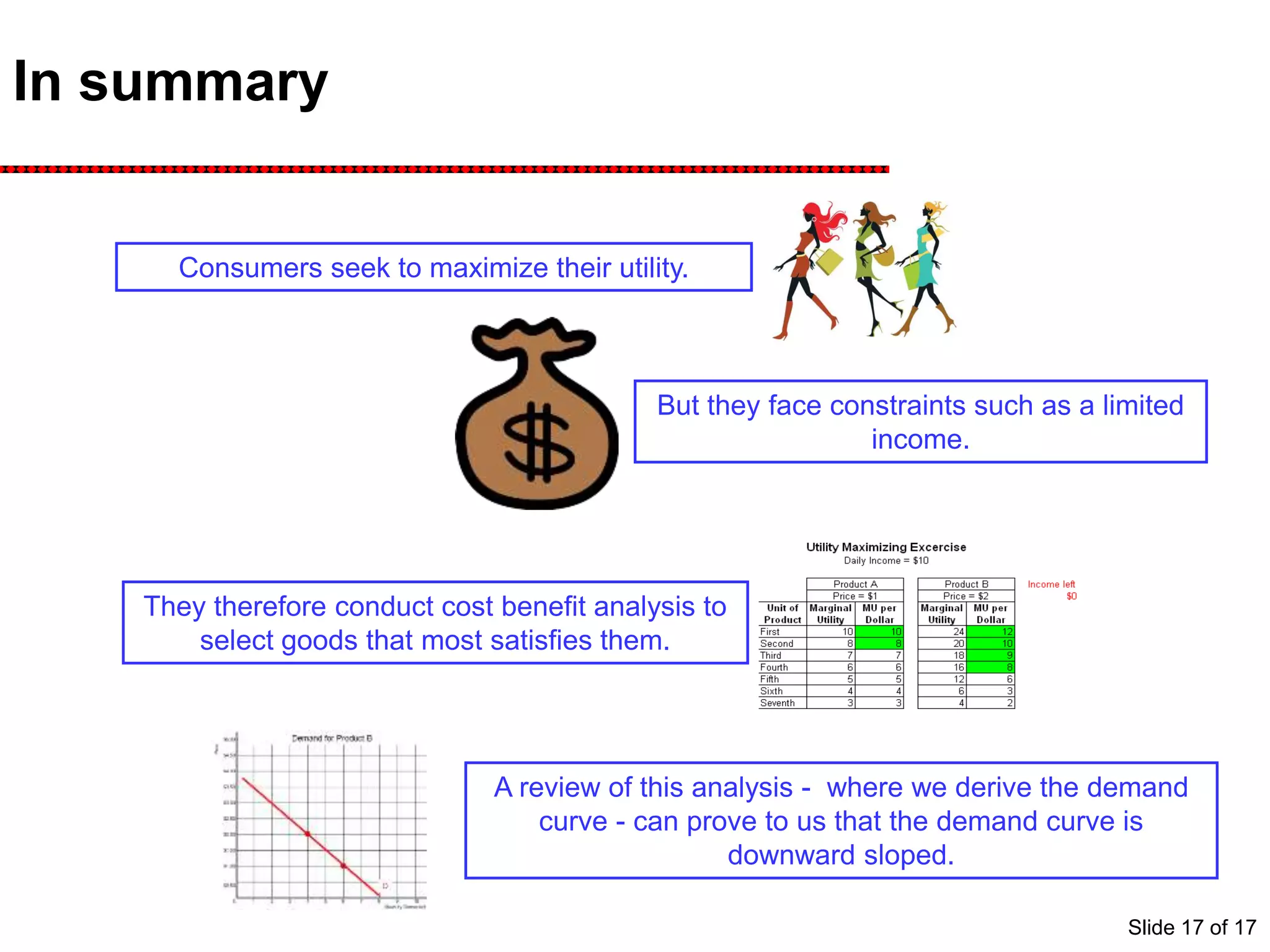
The document discusses the analysis of consumer choice and how to derive the downward sloping demand curve. It introduces concepts like marginal utility, the law of diminishing marginal utility, and utility maximization. An example is used to show how a consumer would make choices between goods A and B under different price scenarios to maximize their utility within their budget. By connecting the quantity chosen at different prices, the individual's demand curve for good B can be plotted, showing a negative slope as predicted by the law of diminishing marginal utility and the substitution and income effects.

1. The Analysis of Consumer Choice
“The golden rule for every business is this: put
yourself in your customer’s place.”
-Orison Swett Marden
Slide 1 of 17

2. A look back on utility
We introduced marginal utility in the previous
module. There we learned that it is the increase in
satisfaction that one obtains from consuming
something.
We explored a new term, “utils” to help quantify how
much we enjoy something.
I realize that this is abstract (even silly?) but we need
such a measurement to conduct analysis…so we
have the “util”.
We also reviewed an important law that will shape
our exploration of consumer choices: the Law of
Diminishing Marginal Utility.
Slide 2 of 17

3. A quick review of diminishing
marginal utility
Just as a reminder, The law of diminishing
marginal utility tells us that we get less
satisfaction from each successive unit we
consume.
In more technical terms, this means that for all goods and
services, the marginal utility curve is downward sloping.
Marginal utility can…and will…eventually
turn negative for all goods and services.
This is easy to imagine if we consider pizza. The first slice
is delicious…marginal utility is high.
The tenth slice…well…I bet you wish you did not eat it as
you feel bloated and overstuffed. For that piece marginal
utility is very low, perhaps even negative.
Slide 3 of 17

4. A Real World Application of
Diminishing Marginal Utility
The concept of marginal utility has impacts in the world
around us.
For example, here we have a newspaper machine. You
put in your money, open the door to see the entire stack
of papers and take one.
This however is a soda machine. Put in your money
and only one unit is dispensed.
Why the difference?
Marginal utility for a news paper drops
quickly. After you read one, it is unlikely
that you will read another one.
That means it is unlikely that you will
take more than one if given access to
all of them. Diminishing marginal utility
sets in quickly.
Diminishing marginal utility does not
set in quickly for sodas. In fact, a
second soda is almost as good as the
first.
If given access to the entire inventory,
what might you be tempted to do? Be
honest!
Therefore, because of the law of diminishing marginal
utility, the soda producers must install much more
sophisticated machinery to sell their products!
Slide 4 of 17

5. Let’s turn our attention to
consumer choice
We know that consumer’s want to
maximize their utility.
We also know that they face
constraints… for example, each of us
only has so much money.
How does a consumer decide what to
buy?
Let’s explore this idea further…and
as we do, we’ll derive the demand
curve.
Slide 5 of 17

6. Deriving the demand curve
Consumer’s face choices among
literally thousand upon thousands of
goods and services.
First the assumptions:
To keep things simple, we’ll assume
that the world has only two goods:
product A and product B.
RealityWhat we will assume
In reality, information is not perfect.
But consumers do the best they can
through Marginal Cost Marginal
Benefit analysis to make themselves
happy.
Consumers allocate their resources
(i.e. spend their money) in a way that
maximizes their utility.
In reality, consumers can save
money or borrow from tomorrow by
charging.
Consumers have limited resources.
Specifically, we will assume that each
consumer has $10 per day to spend
and must spend all of it.
Slide 6 of 17

7. The first unit of B
brings the
consumer 24 utils.
That is 12 utils per
dollar.
Here’s a utility maximizing exercise showing
how consumers might make choices
The Utility Maximizing
Combination is 2 units of A and 4
Units of B.
The first unit of A
brings the
consumer 10 utils.
That is 10 utils per
dollar.
This consumer would
buy a unit of B. It
brings 12 units of
utility per dollar. If
the consumer is
maximizing utility per
dollar, Product B
looks better.
In doing so, this
consumer would be
left with $8.
What would they buy
next?
For the next choice,
each product is
valued at 10 utils per
dollar. It is a tie.
This consumer would
buy a unit of A and
B.
In doing so, this
consumer would be
left with $5.
What would they
buy next?
Next, this consumer
would buy a unit of B.
It brings 9 units of
utility per dollar
versus 8 utils per
dollar for product A.
In doing so, this
consumer would be
left with $3.
What would they buy
next?
The next choice is
also a tie.
This consumer
would buy a unit of
A and B. They
each bring 8 units
of utility per dollar.
In doing so, this
consumer would
be left with $0.
The consumer
has now spent
their $10.
And this
combination of
goods (2 units of
A and 4 units of B)
yields 96 utils.
No other
combination of A
and B that can be
purchased for $10
can exceeds that!
Please remember:
at $2 per unit of B,
this consumer
wanted 4 units of B
Here we see this
consumer has ten
dollars.
We’ll assume that
Product A costs $1 and
Product B cost $2.
Having bought one unit
of B for $2, this
consumer has $8 left to
spend.
Slide 7 of 17

8. Overly analytical?
I realize that it is tough to believe that we all sit
around calculating our “marginal utility per
dollar”?
People do not sit there and say, “I’ll take a
coke because it gives my 10 utils (what
ever that means!).
But trust me. Somewhere in your brain, these
calculations are taking place as you spend all
your time trying to maximize your utility.
Now let’s see what happens if the Price of
B fell to $1.B is on SALE !
Slide 8 of 17

9. Assume the price
of B falls to $1
This table shows a
the hypothetical
consumer’s MU
and MU per dollar
given the new
price.
Assume this
consumer has $10
to spend. What
would they buy?
What if the Price of B fell to $1?
This consumer
would buy a unit of
B. It brings 24
units of utility per
dollar.
In doing so, this
consumer would
be left with $9.
What would they
buy next?
This consumer
would buy another
unit of B. It brings
20 units of utility
per dollar.
In doing so, this
consumer would
be left with $8.
What would they
buy next?
This consumer
would buy another
unit of B. It brings
18 units of utility
per dollar.
In doing so, this
consumer would
be left with $7.
What would they
buy next?
This consumer
would buy another
unit of B. It brings
16 units of utility
per dollar.
In doing so, this
consumer would
be left with $6.
What would they
buy next?
This consumer
would buy another
unit of B. It brings
12 units of utility
per dollar.
In doing so, this
consumer would
be left with $5.
What would they
buy next?
This consumer
would buy a unit of
A. It brings 10
units of utility per
dollar.
In doing so, this
consumer would
be left with $4.
What would they
buy next?
This consumer
would buy a unit of
A. It brings 8 units
of utility per dollar.
In doing so, this
consumer would
be left with $3.
What would they
buy next?
This consumer
would buy a unit of
A. It brings 7 units
of utility per dollar.
In doing so, this
consumer would be
left with $2.
What would this
consumer buy next?
It is a tie.
This consumer
would buy a unit of
A and B. They each
bring 6 units of utility
per dollar.
In doing so, this
consumer would be
left with $0.
This combination
of goods (4 units
of A and 6 units of
B) yields 127 utils.
No other
combination of A
and B that can be
purchased for $10
can exceeds that!
Utility Maximizing Combination is 4
units of A and 6 units of B
Please remember:
at $1, this consumer
wanted 6 units of B
Slide 9 of 17

10. Let’s reflect back to the downward
sloping demand curve
D
Slide 10 of 17

11. Deriving the Demand Curve
When Product B was $2, this
consumer chose to purchase
4 units of B
When the price of Product B
fell to $1, 6 units of B were
purchased!
Connecting those points
may give us this consumer’s
demand curve for this product.
Note it’s downward slope!
D
Demand for Product B
Slide 11 of 17

12. Individual Exercise
I suggest you do this- you will see one of these on the test
Step one: Determine the utility maximizing
combination of A and B with these two scenarios Step two: Graph the demand curve for product B
3.0
Slide 12 of 17

13. Why is the demand curve downward sloped?
• There are 3 primary reasons
– Law of Diminishing Marginal Utility
– Income effect
– Substitution effect
Let’s quickly
explore these
three ideas...
Slide 13 of 17

14. Reason #1: Diminishing Marginal Utility
• As we consume more of an
item, each successive unit
brings us less satisfaction
• Eventually, the marginal cost of
that item outweighs the
marginal utility
Eventually, kids get tired of
swinging. Diminishing marginal
utility sets in!
(Trust me, it takes a long time.)
Slide 14 of 17

15. Reason #2: Income effect
• A fall in the price of a good we
buy means we have more
money to spend
• As prices of a good we buy
decline, our purchasing power
or “real income” increases
(and vice versa). We demand
more of all normal goods.
Slide 15 of 17

16. Reason #3: Substitution effect
A higher price for a good causes us to
demand less of it as we seek to find “a
better buy”
For example, if
butter prices
increased a lot, I
think many of us
would substitute
margarine.
Slide 16 of 17

17. In summary
But they face constraints such as a limited
income.
Consumers seek to maximize their utility.
They therefore conduct cost benefit analysis to
select goods that most satisfies them.
A review of this analysis - where we derive the demand
curve - can prove to us that the demand curve is
downward sloped.
Slide 17 of 17