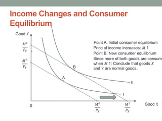
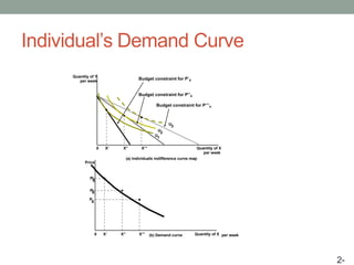
CHAPTER 4
Consumer Behavior
McGraw-Hill/Irwin Copyright © 2014 by The McGraw-Hill Companies, Inc. All rights reserved.
INTRODUCTION
Learning objectives
What will you learn in this module?
 What are the four basic properties of consumer’s
preference?
 How changes in price and income influences individual’s
opportunities?
 Explain the consumer equilibrium point where marginal
rate of substitution is equal to the ratio of prices of two
goods.
• Explain how change in price of a good create substitution
effects and income effects of consumer.
2-3
Consumer Behavior
• A consumer is an individual who purchases goods and
services from firms for the purpose of consumption.
• As a manager of a firm, you are interested not only in who
consumes the good but in who purchases it. The theory of
consumer behaviour helps us to draw individual and
market demand curves.
4-4
Consumer Behaviour
In characterising consumer behaviour, there are two
important factors to consider:
1. Consumer Opportunities
• Consumer opportunities are the set of goods and services that
consumers can afford to consume.
2. Consumer Utility Preferences
• Determine what are the particular goods will be consumed.
2-5
CHAPTER 4
Consumer Behavior
McGraw-Hill/Irwin Copyright © 2014 by The McGraw-Hill Companies, Inc. All rights reserved.
UTILITY PREFERENCES
4 Properties of Utility Preferences
4-8
 Completeness
• Preferences are complete: we assume that an individual
can state which of any two options is preferable.
• Transitivity:
• Preferences are transitive: For any three bundles, , , and : if
A is preferred to B, and B is preferred to C, then A must be
preferred to C
• More is better
• Economic good yields positive benefits to consumer. Thus,
more quantity of a good is always better than less.
• Diminishing marginal rate of substitution
• As an individual will reduce consumption of good Y to get
one more unit of good X
The Indifference Curve
• Definition: An indifference curve is a graph showing
combination of two goods that give the consumer equal
satisfaction and utility. Each point on an indifference curve
indicates that a consumer is indifferent between the two
and all points give him the same utility.
• Description: Graphically, the indifference curve is drawn
as a downward sloping convex to the origin. The graph
shows a combination of two goods that the consumer
consumes.
• 6 hamburgers, 2 soft drinks a week (point A) have equal
satisfaction and utility with 4 hamburgers and 3 soft drinks
a week (point B)
A VIDEO ABOUT
For more information on indifference curve,
please view:
https://www.youtube.com/watch?v=iOmDo5jLFw
8
The Indifference Curve
• Let's take a look at this
figure
2-
6
A
B
C
D
U1
4
3
2
Soft drinks
per week2 3 4 5 60
Hamburgers
per week
The Budget Constraint
• Budget constraint
• Individual’s budget constraint is the limit that a person’s
income places on the combinations of goods and
services that a consumer can buy.
• Budget set:
• Expenditure do no exceed their income M
• Budget line
The consumer's budget constraint shows in Figure: The Budget
Set. The shaded area represents the consumer's budget set or the
opportunity set.
4-
The Budget Constraint
Good 𝑋
Good 𝑌
0
Budget line: 𝑌 =
𝑀
𝑃 𝑌
−
𝑃 𝑋
𝑃 𝑌
𝑋
𝑀
𝑃𝑌
𝑀
𝑃𝑋
𝑃𝑋
𝑃𝑌
Slope
Bundle G
Bundle H
Budget set: 𝑌 ≤
𝑀
𝑃 𝑌
−
𝑃 𝑋
𝑃 𝑌
𝑋
Affordable
Not affordable
A VIDEO ABOUT
For more information on “Budget Constraint”
https://www.youtube.com/watch?v=sNRZE0kwN
GI
The Budget Line
• The slope of the budget line is given by and
represents the market rate of substitution between
goods X and Y. To obtain a better understanding of
the market rate of substitution between goods X
and Y.
Good 𝑋
Good 𝑌
0
Budget line: 𝑌 = 5 −
1
2
𝑋
5
1042
3
4
Market rate of substitution :
4−3
2−4
= −
1
2
Changes in Income
Good 𝑋
Good 𝑌
0
𝑀1
𝑃𝑌
𝑀1
𝑃𝑌
𝑀0
𝑃𝑌
𝑀0
𝑃𝑌
𝑀 ↑
𝑀2
𝑃𝑌
𝑀2
𝑃𝑌
𝑀 ↓
• Individual’s budget depends on
market price and consumer’s income.
• The shift in the budget line
due to the changes in income
of individuals while prices
remain constant.
Changes in Price
Good 𝑋
Good 𝑌
0
New budget line
𝑀
𝑃𝑌
𝑃𝑋
0
> 𝑃𝑋
1
Initial budget
line
𝑀
𝑃𝑋
0
𝑀
𝑃𝑋
1
• The shift in the budget line as
the price of good X decreases
while price of good Y remains
unchanged.
CHAPTER 4
Consumer Behavior
McGraw-Hill/Irwin Copyright © 2014 by The McGraw-Hill Companies, Inc. All rights reserved.
UTILITY MAXIMIZATION
Utility Maximization
• Consumer equilibrium
• the consumer chooses X, Y is the affordable point that lies on (is
tangent to) the highest indifference curve, so it represents utility
maximization.
• marginal rate of substitution (Slope of indifference curve) =
Slope of budget constraint
• The marginal rate of substitution (MRS) can be defined as how
many units of good x have to be given up in order to gain an extra
unit of good y, while keeping the same level of utility. Therefore, it
involves the trade-offs of goods, in order to change the allocation of
bundles of goods while maintaining the same level of satisfaction.
Utility Maximization
Consider a bundle such as A in the
Figure: Consumer Equilibrium. This
combination of Goods X and Y lies on
the budget line, so the cost of Bundle A
completely exhausts the consumer's
income.
A VIDEO ABOUT
For more information on “Utility Maximization”
https://www.youtube.com/watch?v=MXIgp-P-
FeY
Consumer Equilibrium
Good 𝑋
Good 𝑌
0
Consumer equilibrium
A
B
C
I
II
III
D
Change in Consumer Demand
• Price and income changes that influence consumer’s
budget and their level of satisfaction.
• how price and income changes influence consumer
equilibrium.
4-
Price Changes and Consumer
Equilibrium
• Price increases (decreases) reduce (expand) a
consumer’s budget.
• The new consumer equilibrium resulting from a price
change depends on consumer preferences:
• Goods X and Y are:
• substitutes when an increase (decrease) in the price of X leads to an
increase (decrease) in the consumption of Y.
• complements when an increase (decrease) in the price of X leads to a
decrease (increase) in the consumption of Y.
4-
Price Changes and Consumer
Equilibrium
Good 𝑋
Good 𝑌
0
Point A: Initial consumer equilibrium
Price of good X decreases: 𝑃𝑋 ↓
A
B
Point B: New consumer equilibrium
𝑋1
𝑋0
𝑌0
𝑌1
I
II
Since 𝑌1 < 𝑌0 when 𝑃𝑋 ↓:
Conclude that goods 𝑋 and 𝑌 are
substitutes
𝑀
𝑃𝑌
𝑀
𝑃𝑋
1
𝑀
𝑃𝑋
0
Income Changes and Consumer
Equilibrium
• Income increases (decreases) reduce (expand) a
consumer’s budget set.
• The new consumer equilibrium resulting from an income
change depends on consumer preferences:
• Good X is:
• a normal good when an increase (decrease) in income leads to an
increase (decrease) in the consumption of X.
• an inferior good when an increase (decrease) in income leads to a
decrease (increase) in the consumption of X.
4-
Income Changes and Consumer
Equilibrium
Good 𝑋
Good 𝑌
0
A
B
II
I
Point A: Initial consumer equilibrium
Price of income increases: 𝑀 ↑
Point B: New consumer equilibrium
Since more of both goods are consume
when 𝑀 ↑: Conclude that goods 𝑋
and 𝑌 are normal goods.
𝑀0
𝑃𝑋
𝑀1
𝑃𝑋
𝑀0
𝑃𝑌
𝑀1
𝑃𝑌
Substitution and Income Effect
• Part of the change in the quantity demanded for other
goods is caused by the substitution of one good for
another: called substitution effect
• Price change creates difference in real purchasing power;
consumers move to a new indifference curve consistent
with their new purchasing power
• Part of the change in the quantity demanded is caused by
the change in real income: called income effect.
2-
Substitution and Income Effects
Good 𝑋
Good 𝑌
0
Point A: Initial consumer equilibrium
Price of good X increases: 𝑃𝑋 ↑
C A
Point B: substitution effect
𝑋0𝑋1 𝑋 𝑀
B
Point C: income effect and new
consumer equilibrium
Substitution
effect
Income
effect
I G
H
F
J
CHAPTER 4
Consumer Behavior
McGraw-Hill/Irwin Copyright © 2014 by The McGraw-Hill Companies, Inc. All rights reserved.
CONSUMER DEMAND
Consumer Demand
• The indifference curves and consumers’ reactions to
changes in prices and income are the basis of the
demand functions
• Relationship between Indifference Curves and Demand
Curves.
• Individual's Demand Curve is to see where the demand
curve for normal goods come from.
• The consumer initially is in equilibrium at Point X’, where
income is fixed and prices at and Pox.
4-
Individual’s Demand Curve
• But when the price of good X falls to the lower level P1x,
the opportunity expands and the consumer reaches a
new equilibrium at Point.
• You may see the relationship between the price of good X
and the quantity consumed of good X is graphed in the
Figure (b) and is individual consumer's demand curve for
good X.
Individual’s Demand Curve
2-
Quantity of Y
per week
U1
U2
U3
X
Quantity of X
per week
X’ X” X’”
(a) Individual’s indifference curve map
0
Price
P9
XP0
X
P-
Quantity of X per weekX’ X” X’” (b) Demand curve0
Budget constraint for P’X
Budget constraint for P’’X
Budget constraint for P’’’X
Market Demand
we can derive market demand curve based on two individuals
2-
(a) Individual 1
PX
X
P*
X*
1
0
(b) Individual 2
X*
2
0
(c) Market Demand
X
D
X*0
PX PX
CHAPTER 4
Market Forces: Demand and Supply
RECAP
On Key Terms and Concepts
2-38
Key Concepts Chapter 4
• Indifference curve properties
• Consumer preferences
• Budget constraint
• Budget line
• Marginal Rate of Substitution
• Substitution effects
• Income effects
• Normal goods and Inferior goods
• Individual Demand
• Market demand.
4-

Chapter 4 Consumer Behavior

  • 1.
    CHAPTER 4 Consumer Behavior McGraw-Hill/IrwinCopyright © 2014 by The McGraw-Hill Companies, Inc. All rights reserved.
  • 2.
  • 3.
    Learning objectives What willyou learn in this module?  What are the four basic properties of consumer’s preference?  How changes in price and income influences individual’s opportunities?  Explain the consumer equilibrium point where marginal rate of substitution is equal to the ratio of prices of two goods. • Explain how change in price of a good create substitution effects and income effects of consumer. 2-3
  • 4.
    Consumer Behavior • Aconsumer is an individual who purchases goods and services from firms for the purpose of consumption. • As a manager of a firm, you are interested not only in who consumes the good but in who purchases it. The theory of consumer behaviour helps us to draw individual and market demand curves. 4-4
  • 5.
    Consumer Behaviour In characterisingconsumer behaviour, there are two important factors to consider: 1. Consumer Opportunities • Consumer opportunities are the set of goods and services that consumers can afford to consume. 2. Consumer Utility Preferences • Determine what are the particular goods will be consumed. 2-5
  • 6.
    CHAPTER 4 Consumer Behavior McGraw-Hill/IrwinCopyright © 2014 by The McGraw-Hill Companies, Inc. All rights reserved.
  • 7.
  • 8.
    4 Properties ofUtility Preferences 4-8  Completeness • Preferences are complete: we assume that an individual can state which of any two options is preferable. • Transitivity: • Preferences are transitive: For any three bundles, , , and : if A is preferred to B, and B is preferred to C, then A must be preferred to C • More is better • Economic good yields positive benefits to consumer. Thus, more quantity of a good is always better than less. • Diminishing marginal rate of substitution • As an individual will reduce consumption of good Y to get one more unit of good X
  • 9.
    The Indifference Curve •Definition: An indifference curve is a graph showing combination of two goods that give the consumer equal satisfaction and utility. Each point on an indifference curve indicates that a consumer is indifferent between the two and all points give him the same utility. • Description: Graphically, the indifference curve is drawn as a downward sloping convex to the origin. The graph shows a combination of two goods that the consumer consumes. • 6 hamburgers, 2 soft drinks a week (point A) have equal satisfaction and utility with 4 hamburgers and 3 soft drinks a week (point B)
  • 10.
    A VIDEO ABOUT Formore information on indifference curve, please view: https://www.youtube.com/watch?v=iOmDo5jLFw 8
  • 11.
    The Indifference Curve •Let's take a look at this figure 2- 6 A B C D U1 4 3 2 Soft drinks per week2 3 4 5 60 Hamburgers per week
  • 12.
    The Budget Constraint •Budget constraint • Individual’s budget constraint is the limit that a person’s income places on the combinations of goods and services that a consumer can buy. • Budget set: • Expenditure do no exceed their income M • Budget line The consumer's budget constraint shows in Figure: The Budget Set. The shaded area represents the consumer's budget set or the opportunity set. 4-
  • 13.
    The Budget Constraint Good𝑋 Good 𝑌 0 Budget line: 𝑌 = 𝑀 𝑃 𝑌 − 𝑃 𝑋 𝑃 𝑌 𝑋 𝑀 𝑃𝑌 𝑀 𝑃𝑋 𝑃𝑋 𝑃𝑌 Slope Bundle G Bundle H Budget set: 𝑌 ≤ 𝑀 𝑃 𝑌 − 𝑃 𝑋 𝑃 𝑌 𝑋 Affordable Not affordable
  • 14.
    A VIDEO ABOUT Formore information on “Budget Constraint” https://www.youtube.com/watch?v=sNRZE0kwN GI
  • 15.
    The Budget Line •The slope of the budget line is given by and represents the market rate of substitution between goods X and Y. To obtain a better understanding of the market rate of substitution between goods X and Y. Good 𝑋 Good 𝑌 0 Budget line: 𝑌 = 5 − 1 2 𝑋 5 1042 3 4 Market rate of substitution : 4−3 2−4 = − 1 2
  • 16.
    Changes in Income Good𝑋 Good 𝑌 0 𝑀1 𝑃𝑌 𝑀1 𝑃𝑌 𝑀0 𝑃𝑌 𝑀0 𝑃𝑌 𝑀 ↑ 𝑀2 𝑃𝑌 𝑀2 𝑃𝑌 𝑀 ↓ • Individual’s budget depends on market price and consumer’s income. • The shift in the budget line due to the changes in income of individuals while prices remain constant.
  • 17.
    Changes in Price Good𝑋 Good 𝑌 0 New budget line 𝑀 𝑃𝑌 𝑃𝑋 0 > 𝑃𝑋 1 Initial budget line 𝑀 𝑃𝑋 0 𝑀 𝑃𝑋 1 • The shift in the budget line as the price of good X decreases while price of good Y remains unchanged.
  • 18.
    CHAPTER 4 Consumer Behavior McGraw-Hill/IrwinCopyright © 2014 by The McGraw-Hill Companies, Inc. All rights reserved.
  • 19.
  • 20.
    Utility Maximization • Consumerequilibrium • the consumer chooses X, Y is the affordable point that lies on (is tangent to) the highest indifference curve, so it represents utility maximization. • marginal rate of substitution (Slope of indifference curve) = Slope of budget constraint • The marginal rate of substitution (MRS) can be defined as how many units of good x have to be given up in order to gain an extra unit of good y, while keeping the same level of utility. Therefore, it involves the trade-offs of goods, in order to change the allocation of bundles of goods while maintaining the same level of satisfaction.
  • 21.
    Utility Maximization Consider abundle such as A in the Figure: Consumer Equilibrium. This combination of Goods X and Y lies on the budget line, so the cost of Bundle A completely exhausts the consumer's income.
  • 22.
    A VIDEO ABOUT Formore information on “Utility Maximization” https://www.youtube.com/watch?v=MXIgp-P- FeY
  • 23.
    Consumer Equilibrium Good 𝑋 Good𝑌 0 Consumer equilibrium A B C I II III D
  • 24.
    Change in ConsumerDemand • Price and income changes that influence consumer’s budget and their level of satisfaction. • how price and income changes influence consumer equilibrium. 4-
  • 25.
    Price Changes andConsumer Equilibrium • Price increases (decreases) reduce (expand) a consumer’s budget. • The new consumer equilibrium resulting from a price change depends on consumer preferences: • Goods X and Y are: • substitutes when an increase (decrease) in the price of X leads to an increase (decrease) in the consumption of Y. • complements when an increase (decrease) in the price of X leads to a decrease (increase) in the consumption of Y. 4-
  • 26.
    Price Changes andConsumer Equilibrium Good 𝑋 Good 𝑌 0 Point A: Initial consumer equilibrium Price of good X decreases: 𝑃𝑋 ↓ A B Point B: New consumer equilibrium 𝑋1 𝑋0 𝑌0 𝑌1 I II Since 𝑌1 < 𝑌0 when 𝑃𝑋 ↓: Conclude that goods 𝑋 and 𝑌 are substitutes 𝑀 𝑃𝑌 𝑀 𝑃𝑋 1 𝑀 𝑃𝑋 0
  • 27.
    Income Changes andConsumer Equilibrium • Income increases (decreases) reduce (expand) a consumer’s budget set. • The new consumer equilibrium resulting from an income change depends on consumer preferences: • Good X is: • a normal good when an increase (decrease) in income leads to an increase (decrease) in the consumption of X. • an inferior good when an increase (decrease) in income leads to a decrease (increase) in the consumption of X. 4-
  • 28.
    Income Changes andConsumer Equilibrium Good 𝑋 Good 𝑌 0 A B II I Point A: Initial consumer equilibrium Price of income increases: 𝑀 ↑ Point B: New consumer equilibrium Since more of both goods are consume when 𝑀 ↑: Conclude that goods 𝑋 and 𝑌 are normal goods. 𝑀0 𝑃𝑋 𝑀1 𝑃𝑋 𝑀0 𝑃𝑌 𝑀1 𝑃𝑌
  • 29.
    Substitution and IncomeEffect • Part of the change in the quantity demanded for other goods is caused by the substitution of one good for another: called substitution effect • Price change creates difference in real purchasing power; consumers move to a new indifference curve consistent with their new purchasing power • Part of the change in the quantity demanded is caused by the change in real income: called income effect. 2-
  • 30.
    Substitution and IncomeEffects Good 𝑋 Good 𝑌 0 Point A: Initial consumer equilibrium Price of good X increases: 𝑃𝑋 ↑ C A Point B: substitution effect 𝑋0𝑋1 𝑋 𝑀 B Point C: income effect and new consumer equilibrium Substitution effect Income effect I G H F J
  • 31.
    CHAPTER 4 Consumer Behavior McGraw-Hill/IrwinCopyright © 2014 by The McGraw-Hill Companies, Inc. All rights reserved.
  • 32.
  • 33.
    Consumer Demand • Theindifference curves and consumers’ reactions to changes in prices and income are the basis of the demand functions • Relationship between Indifference Curves and Demand Curves. • Individual's Demand Curve is to see where the demand curve for normal goods come from. • The consumer initially is in equilibrium at Point X’, where income is fixed and prices at and Pox. 4-
  • 34.
    Individual’s Demand Curve •But when the price of good X falls to the lower level P1x, the opportunity expands and the consumer reaches a new equilibrium at Point. • You may see the relationship between the price of good X and the quantity consumed of good X is graphed in the Figure (b) and is individual consumer's demand curve for good X.
  • 35.
    Individual’s Demand Curve 2- Quantityof Y per week U1 U2 U3 X Quantity of X per week X’ X” X’” (a) Individual’s indifference curve map 0 Price P9 XP0 X P- Quantity of X per weekX’ X” X’” (b) Demand curve0 Budget constraint for P’X Budget constraint for P’’X Budget constraint for P’’’X
  • 36.
    Market Demand we canderive market demand curve based on two individuals 2- (a) Individual 1 PX X P* X* 1 0 (b) Individual 2 X* 2 0 (c) Market Demand X D X*0 PX PX
  • 37.
    CHAPTER 4 Market Forces:Demand and Supply
  • 38.
    RECAP On Key Termsand Concepts 2-38
  • 39.
    Key Concepts Chapter4 • Indifference curve properties • Consumer preferences • Budget constraint • Budget line • Marginal Rate of Substitution • Substitution effects • Income effects • Normal goods and Inferior goods • Individual Demand • Market demand. 4-