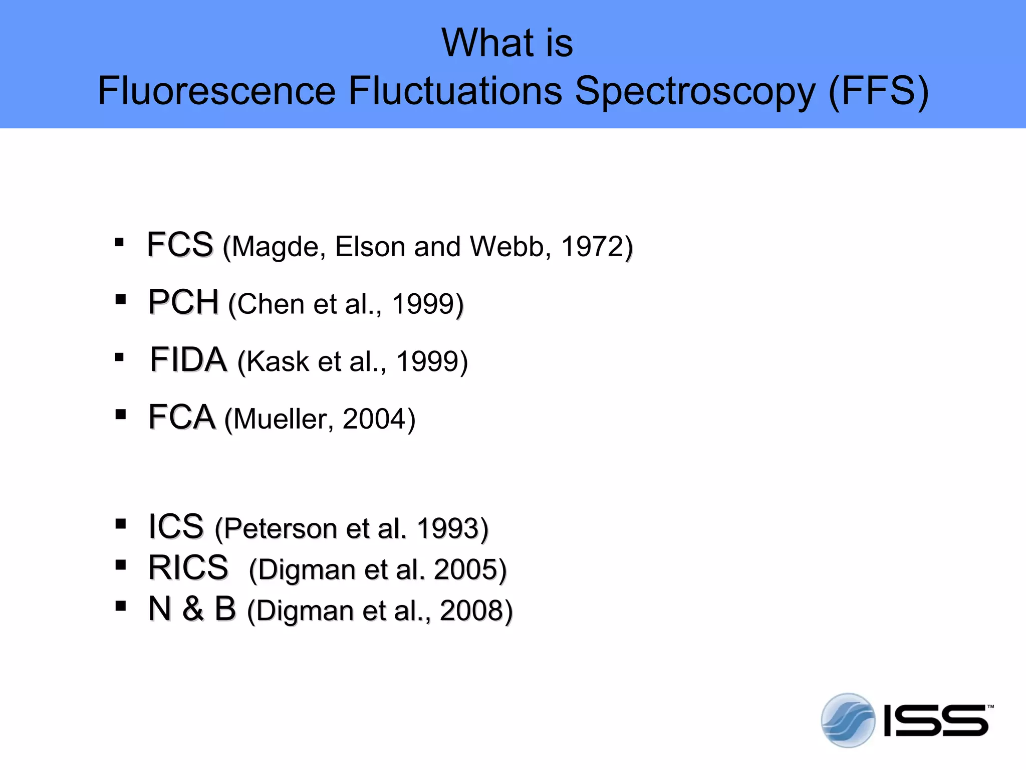
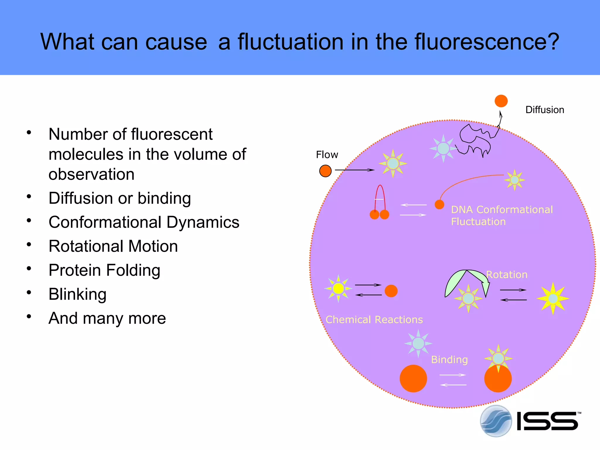
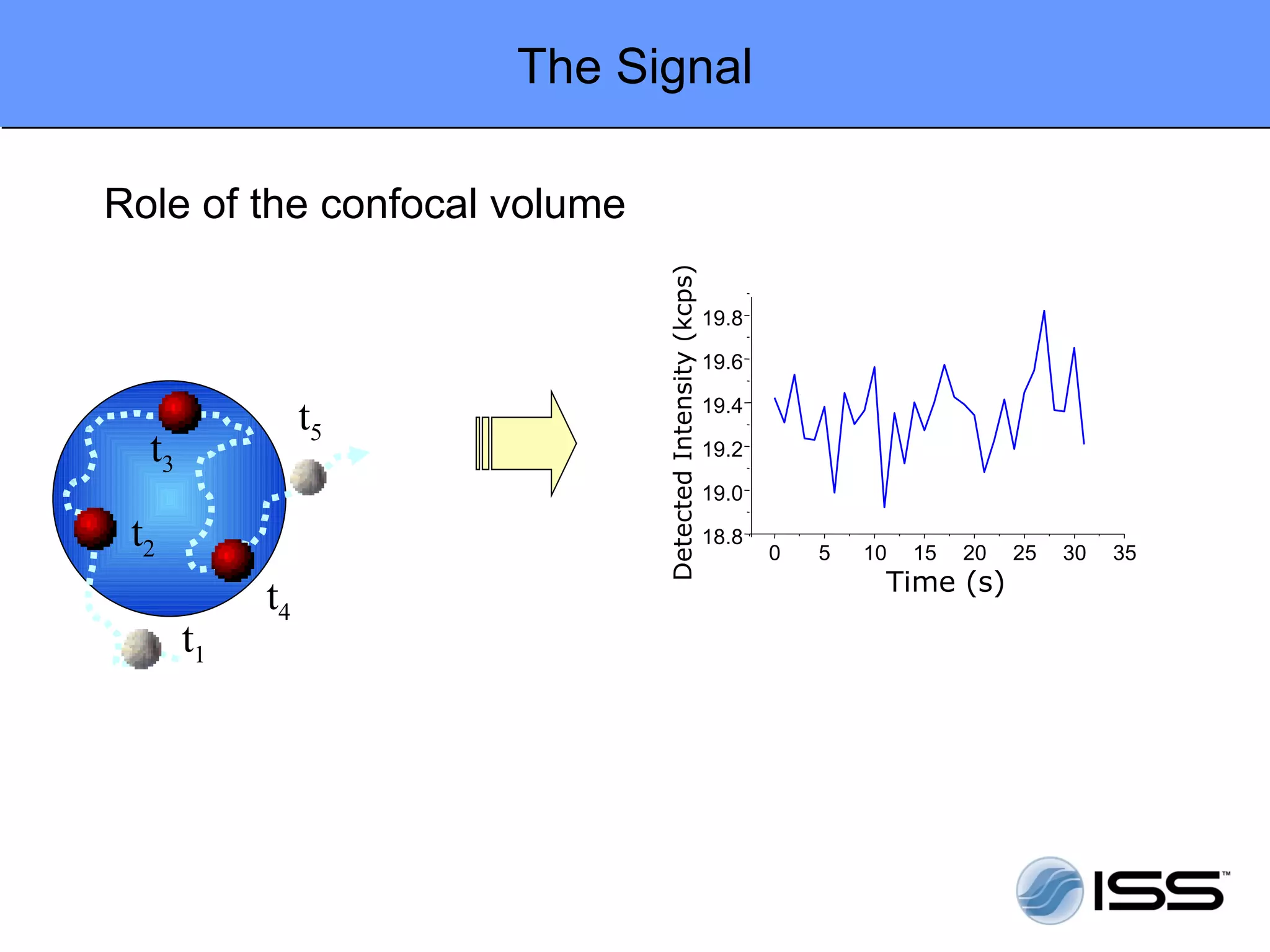
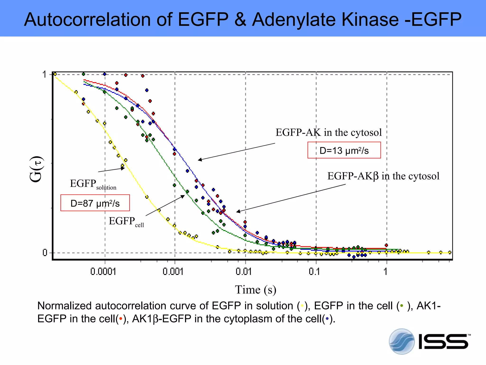
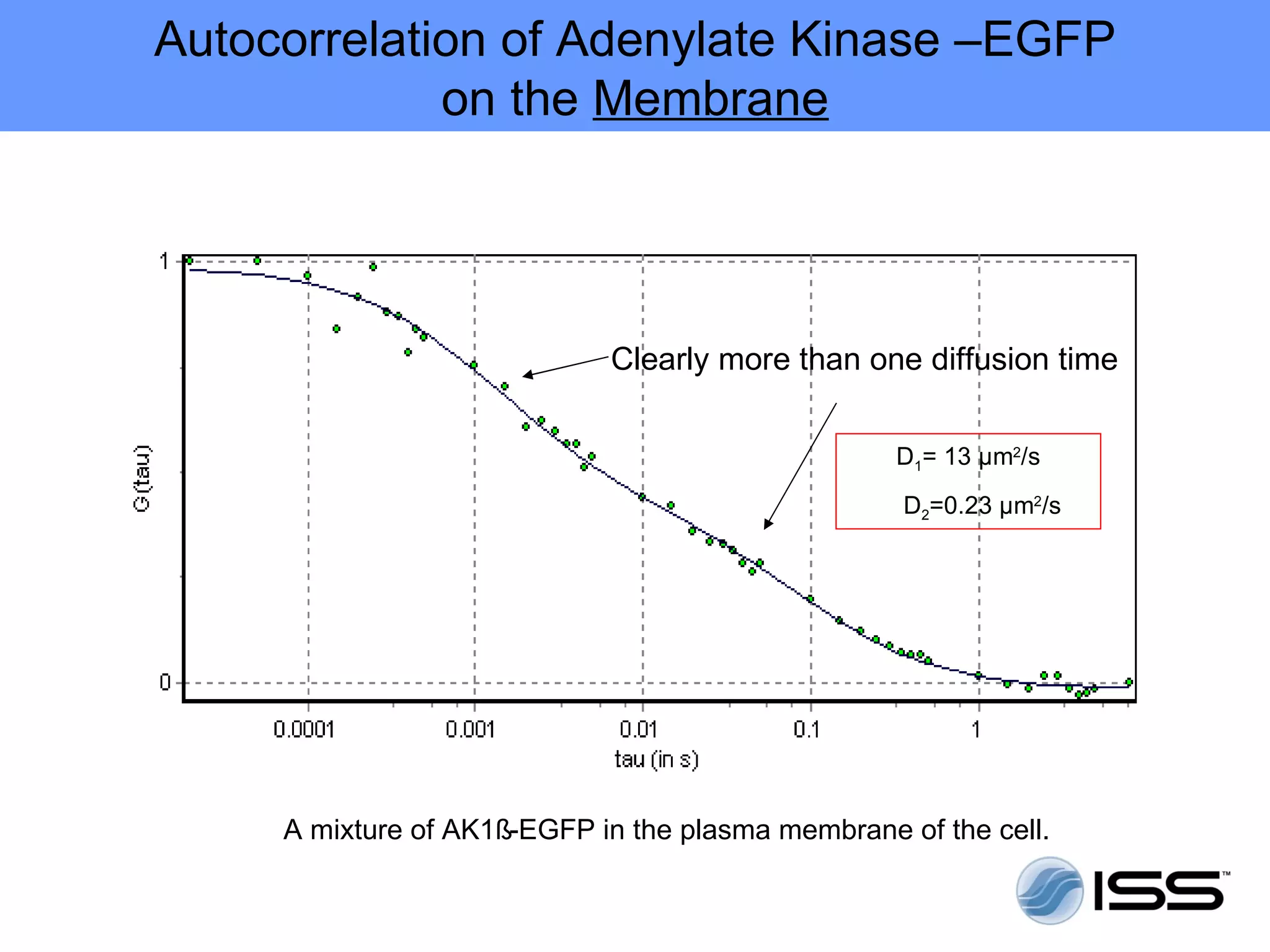
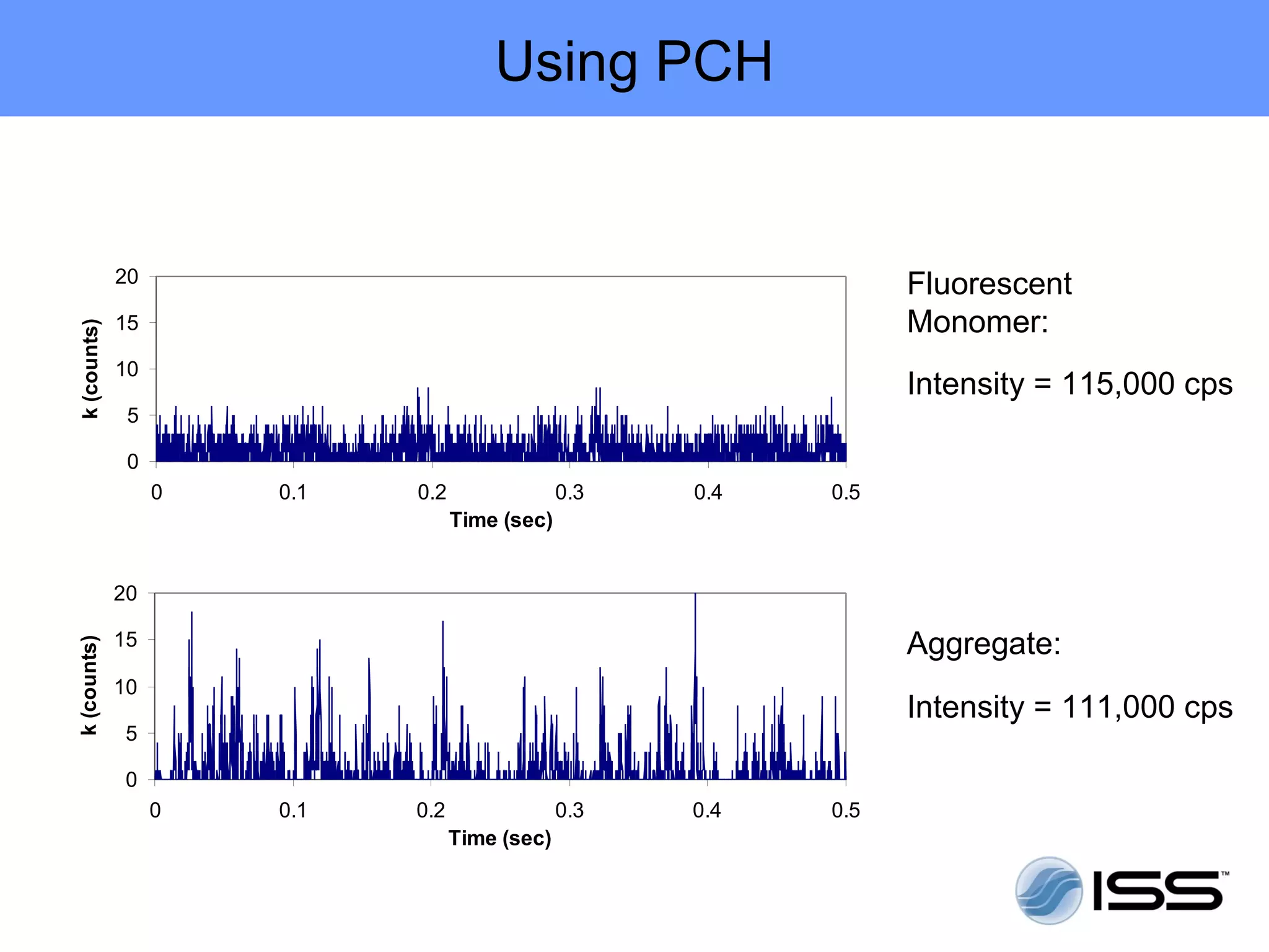
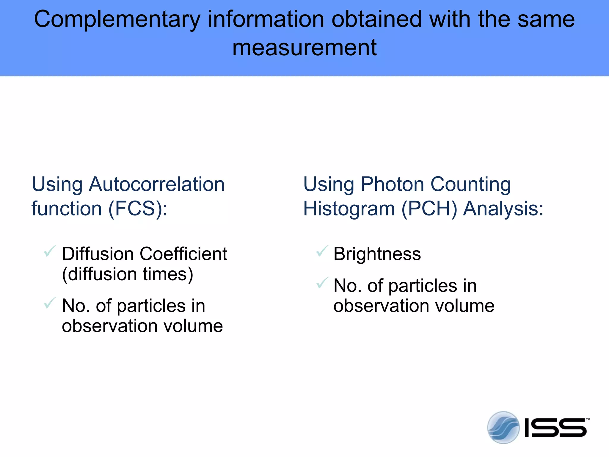
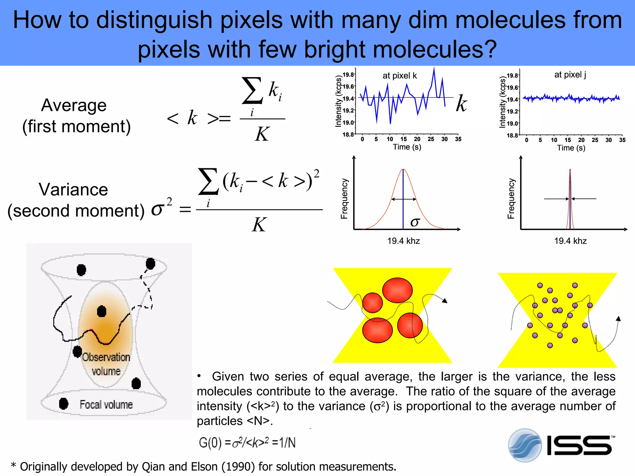
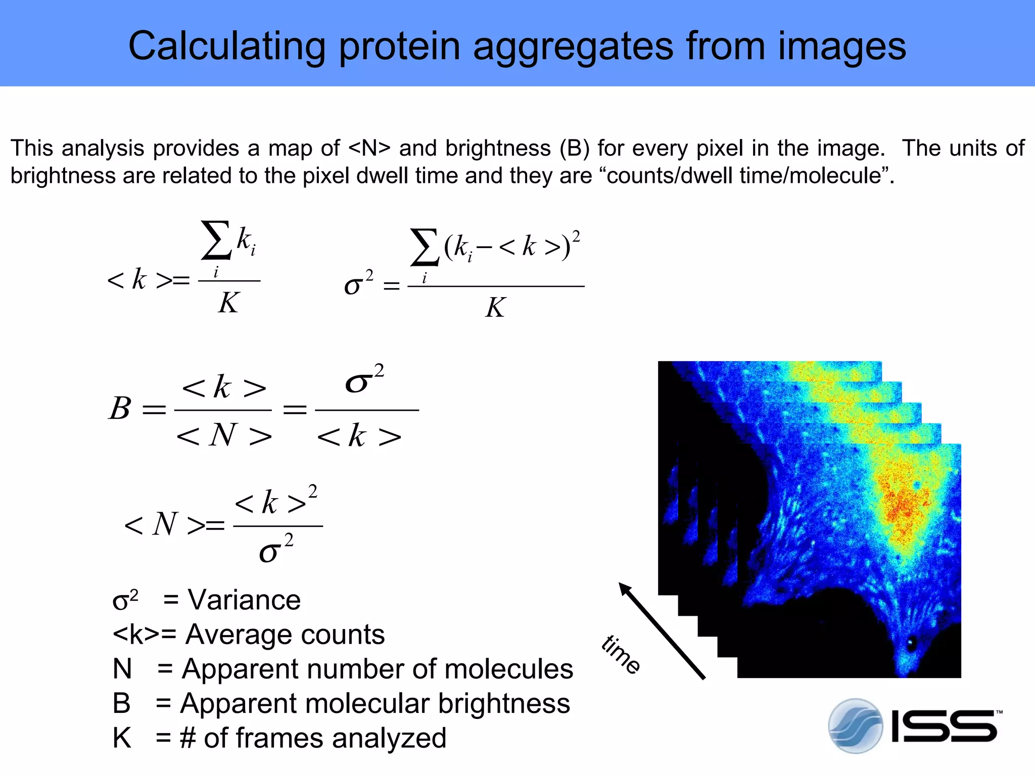
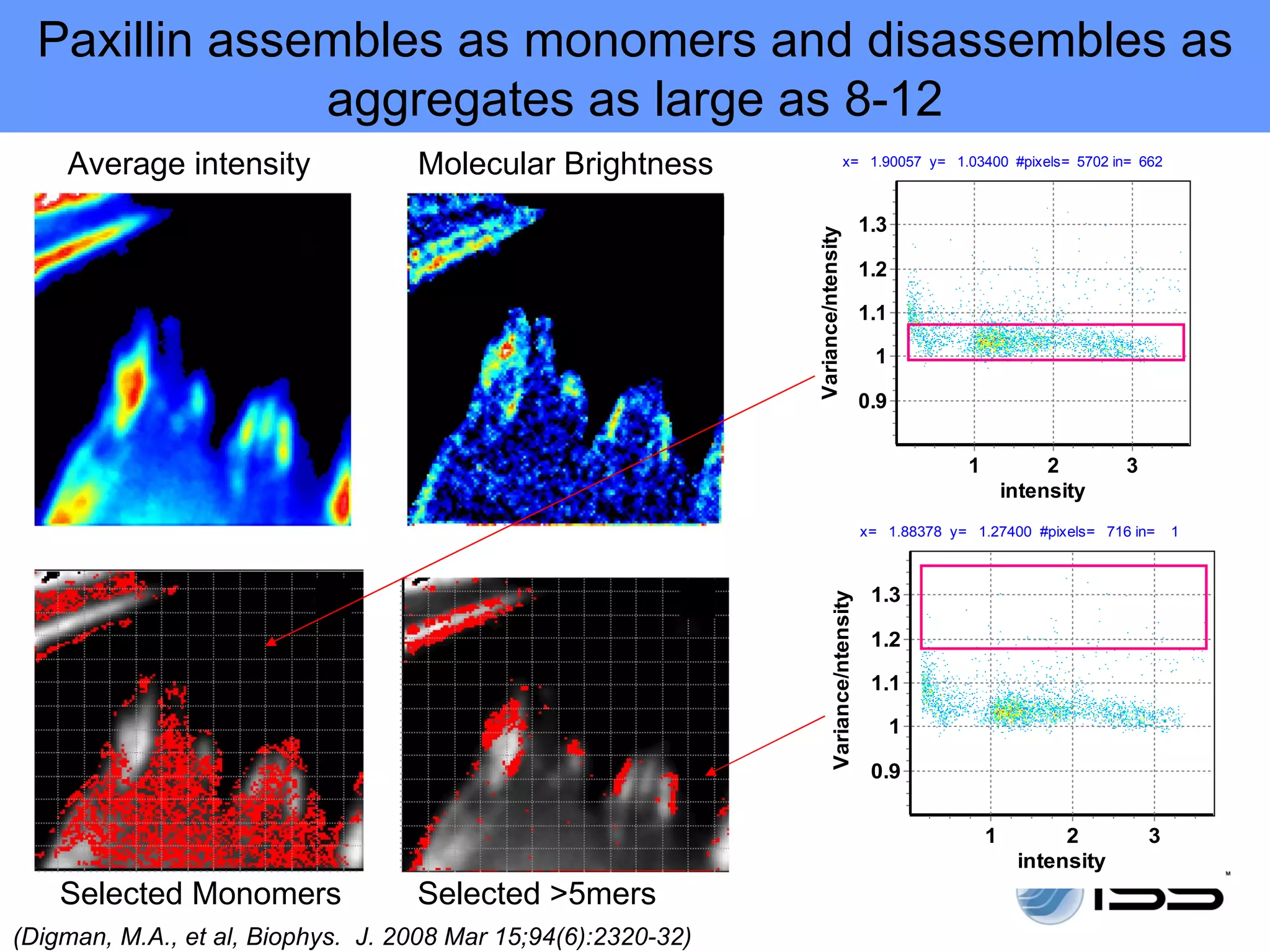
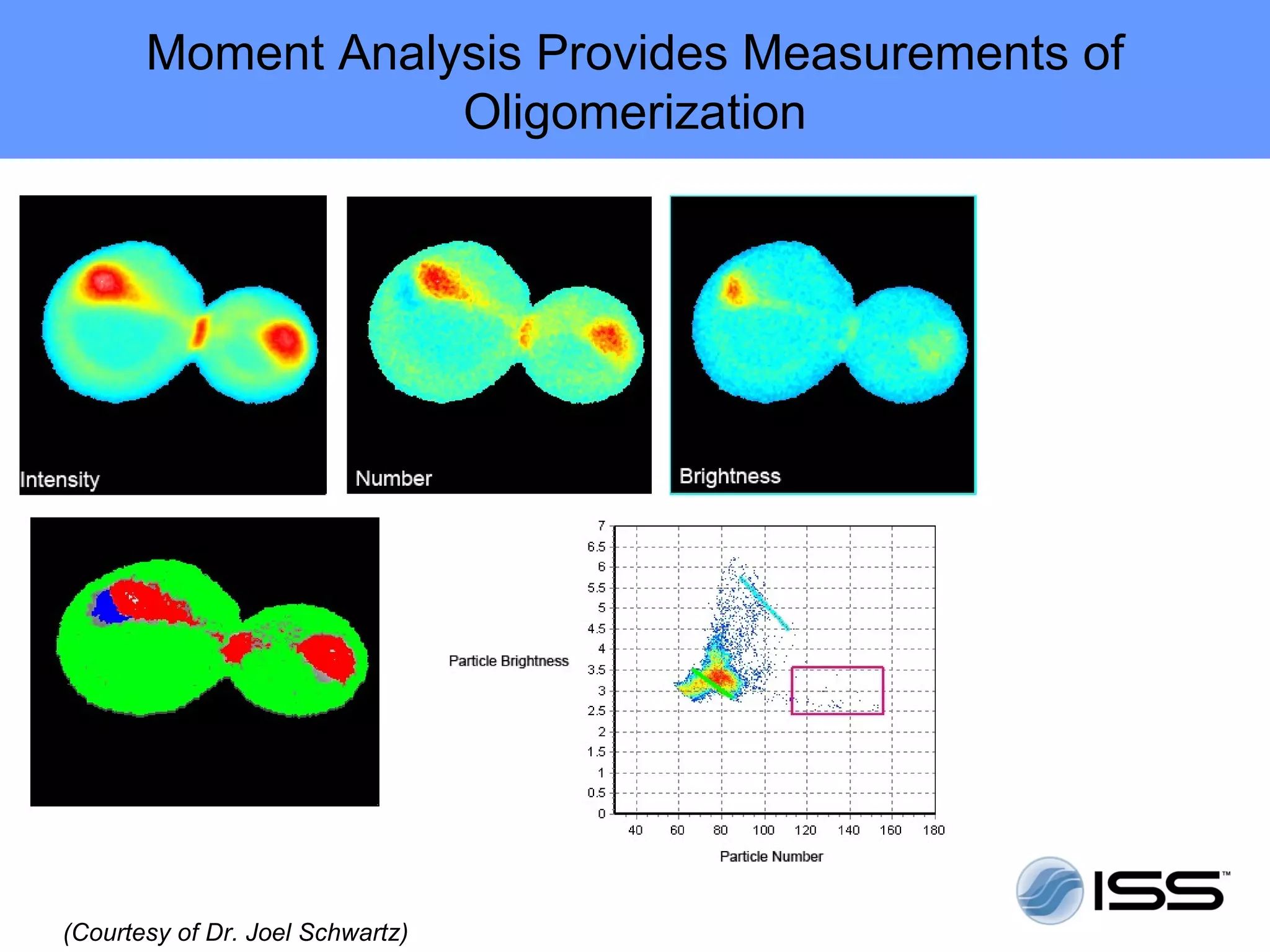
2. Alba FFS/FLIM confocal microscope
Applications in Biology

3. Cell Images

4. Moving from Images to Spectroscopy

5. Confocal microscopy: FFS & FLIM
Alba confocal microscope and FFS/FLIM spectrometer

6. Alba, 4-channel unit schematics

7. What is
Fluorescence Fluctuations Spectroscopy (FFS)
 FCS (Magde, Elson and Webb, 1972)
(
 PCH (Chen et al., 1999)
(
 FIDA (Kask et al., 1999)
 FCA (Mueller, 2004)
(
 ICS (Peterson et al. 1993)
 RICS (Digman et al. 2005)
 N & B (Digman et al., 2008)

8. What can cause a fluctuation in the fluorescence?
Diffusion
• Number of fluorescent
molecules in the volume of Flow
observation
• Diffusion or binding
DNA Conformational
• Conformational Dynamics Fluctuation
• Rotational Motion
• Protein Folding Rotation
• Blinking
• And many more Chemical Reactions
Binding

9. The Signal
Role of the confocal volume
Detected Intensity (kcps)
19.8
19.6
19.4
t5
t3 19.2
19.0
t2 18.8
0 5 10 15 20 25 30 35
Time (s)
t4
t1

10. How to extract the information about the fluctuations and
their characteristic time?
Distribution of the duration of the fluctuations
Distribution of the amplitude of the fluctuations
To extract the distribution of the duration of the fluctuations we
use a math based on calculation of the correlation function
To extract the distribution of the amplitude of the fluctuations,
we use a math based on the PCH distribution

11. The definition of the Autocorrelation Function
δF(t)δF(t + τ )
δF (t ) = F (t ) − F (t ) G( τ) = 2
F(t)
3
26x10
Fluorescence
Photon Counts
24
22
20
18
16
14
time
12
0 5 10 15 20 25 30 35
Time
τ Average Fluorescence
t t+τ

12. Data Presentation and Analysis
Autocorrelation function: <N> and D
PCH parameters: <N> and ε
<N>: no. of particles in the observation
volume
D: diffusion coefficient
ε: brightness

13. Autocorrelation Adenylate Kinase -EGFP
Chimeric Protein in HeLa Cells
Fluorescence Intensity
Examples of different HeLa cells transfected with AK1-EGFP
Examples of different HeLa cells transfected with AK1β -EGFP
Qiao Qiao Ruan, Y. Chen, E. Gratton, M. Glaser & W. Mantulin; Biophys. J. 83 (2002)

14. Autocorrelation of EGFP & Adenylate Kinase -EGFP
EGFP-AK in the cytosol
D=13 µm2/s
G(τ)
EGFP-AKβ in the cytosol
EGFPsolution
D=87 µm2/s
EGFPcell
Time (s)
Normalized autocorrelation curve of EGFP in solution (•), EGFP in the cell (• ), AK1-
EGFP in the cell(•), AK1β-EGFP in the cytoplasm of the cell(•).

15. Autocorrelation of Adenylate Kinase –EGFP
on the Membrane
Clearly more than one diffusion time
D1= 13 µm2/s
D2=0.23 µm2/s
A mixture of AK1ß-EGFP in the plasma membrane of the cell.

16. Using PCH
20 Fluorescent
15 Monomer:
k (counts)
10
Intensity = 115,000 cps
5
0
0 0.1 0.2 0.3 0.4 0.5
Time (sec)
20
15 Aggregate:
k (counts)
10
Intensity = 111,000 cps
5
0
0 0.1 0.2 0.3 0.4 0.5
Time (sec)

17. Photon Count Histogram (PCH)
1.E+05 1.E+05 1.E+05
log(occurences)
1.E+04 1.E+04 1.E+04
log(occurences)
1.E+03 log(occurences) 1.E+03 1.E+03
1.E+02 1.E+02 1.E+02
1.E+01 1.E+01 1.E+01
1.E+00 1.E+00 1.E+00
0 3 6 9 12 15 18 21 24 0 3 6 9 12 15 18 21 24 0 3 6 9 12 15 18 21 24
k (counts) k (counts) k (counts)
Can we quantitate this?
What contributes to the distribution of intensities?

18. Complementary information obtained with the same
measurement
Using Autocorrelation Using Photon Counting
function (FCS): Histogram (PCH) Analysis:
 Diffusion Coefficient  Brightness
(diffusion times)
 No. of particles in
 No. of particles in observation volume
observation volume

19. What about … ?
• In a cell we may want to locate the areas where we have
clusters of molecules versus single molecules.
• In cells, both the concentration and the clustering of proteins
can differ in various locations and change during biological
processes.
• Number & Brightness (N&B) measures the average number
of molecules and brightness in each pixel of an image.

20. The Number and Brightness (N&B) analysis
Purpose: Provide a pixel resolution map of molecular number and
aggregation in cells
Method: First and second moment of the fluorescence intensity distribution
at each pixel
Source: Raster scanned image obtained with laser scanning microscopes
Output: The N and B maps, B vs intensity 2D histogram

21. How to distinguish pixels with many dim molecules from
pixels with few bright molecules?
∑k
19.8 at pixel k 19.8 at pixel j
Intensity (kcps)
Intensity (kcps)
19.6 19.6
Average
i 19.4
k 19.4
< k >= i 19.2 19.2
(first moment) K
19.0
18.8
0 5 10 15 20 25 30 35
19.0
18.8
0 5 10 15 20 25 30 35
Time (s) Time (s)
∑ ( ki − < k >) 2
Frequency
Frequency
Variance
(second moment) σ =
2 i
K σ
19.4 khz 19.4 khz
• Given two series of equal average, the larger is the variance, the less
molecules contribute to the average. The ratio of the square of the average
intensity (<k>2) to the variance (σ2) is proportional to the average number of
particles <N>.
* Originally developed by Qian and Elson (1990) for solution measurements.

22. Calculating protein aggregates from images
This analysis provides a map of <N> and brightness (B) for every pixel in the image. The units of
brightness are related to the pixel dwell time and they are “counts/dwell time/molecule”.
∑k i ∑ ( k − < k >)
i
2
< k >= i
σ2 = i
K K
<k > σ2
B= =
<N > <k >
< k >2
< N >=
σ2
σ2 = Variance
<k>= Average counts tim
N = Apparent number of molecules e
B = Apparent molecular brightness
K = # of frames analyzed

23. Selecting the dwell time
To increase the apparent brightness we could increase the dwell
time, since the brightness is measured in counts/dwell
time/molecule.
Increasing the dwell time decreases the amplitude of the
fluctuation.
1 µs dwell time 1 ms dwell time

24. What contributes to the variance?
Variance due to particle number fluctuations σ =ε n
2
n
2
Variance due to detector shot noise σ = εn
2
d
The measured variance contains two terms, the variance due to the particle
number fluctuation and the variance due to the detector count statistics
noise
These two terms have different dependence on the
molecular brightness:
σ 2 = σ2 + σ2
n d
σ n = ε 2n
2
σ d = εn
2
(for the photon counting detector)
Both depend on the intrinsic brightness and the number of molecules. We can
invert the equations and obtain n and ε
n is the true number of molecules
ε is the true molecular brightness

25. How to Calculate n and ε
σ σn σd ε n σd
2 2 2 2 2
B= = + = + = ε +1
< k > < k > < k > εn < k >
This ratio identifies pixels of different brightness due to mobile particles.
The “true” number of molecules n and the “true” molecular brightness for
mobile particles can be obtained from
< k >2 σ 2− < k >
n= 2 ε=
σ −<k > <k >
If there are regions of immobile particles, n cannot be calculated because for
the immobile fraction the variance is = <k>. For this reason, several plots are
offered to help the operator to identify regions of mobile and immobile
particles. Particularly useful is the plot of NvsB.

26. The effect of the immobile part: with photon counting
detectors (Fluorescent beads in a sea of 100nM Fluorescein).
Intensity B map x= 2.00000 y= 2.00000 #pixels= 0 in= 0
4
3.5 Monomer-octamer seri
3
Variance/ntensity
2.5
4
2
Selecting
3
fluorescein 1.5
2
B
1 Immobile
1
0.5
0
100 200 300
intensity
0
0 1 2 3 4
4
intensity
Selecting
3
beads
2
B
1
0
100 200 300
intensity

27. Paxillin assembles as monomers and disassembles as
aggregates as large as 8-12
Average intensity Molecular Brightness x= 1.90057 y= 1.03400 #pixels= 5702 in= 662
1.3
Variance/ntensity
1.2
1.1
1
0.9
1 2 3
intensity
x= 1.88378 y= 1.27400 #pixels= 716 in= 1
1.3
Variance/ntensity
1.2
1.1
1
0.9
1 2 3
intensity
Selected Monomers Selected >5mers
(Digman, M.A., et al, Biophys. J. 2008 Mar 15;94(6):2320-32)

28. Moment Analysis Provides Measurements of
Oligomerization
(Courtesy of Dr. Joel Schwartz)

29. What about Fluorescence Lifetime Imaging?
FLIM is extensively used for the measurement of parameters
in cells; for instance:
• O2 concentrations in cells or in tissues
• Intracellular mapping of ion concentration and pH imaging
• Biochemical reactions (oxidation/reduction) processes
NAD and NADH
• FRET – Dynamic interactions of molecular species on the
nm scale

30. Perrin-Jablonski diagram

31. Applications of FRET
FRET strongly depends on the distance between the donor and acceptor:
Förster calculated the rate of transfer to be
6
1  R0 
kT =  R
τD  
tD is the lifetime of the donor in the absence of the acceptor.
R is the distance between the two groups
Ro is called the Förster distance
τD
E =1−
τA

32. FRET
Images of opossum kidney cells
expressing a CFP (left column) and
CFP/YFP tandem protein (right
column).
Top: intensity
Bottom: phase lifetime
Left: 2.1 ns; Right: 1.5 ns
Images obtained in frequency domain:
Ti-Sapphire – 2-photon exc. at 850 nm
The images in channel 1 were collected
through a 520 – 560 nm YFP filter and
in channel 2 through a 460 – 500 nm
CFP filter.
Courtesy of Dr. Moshe Levi

33. Applications to Cerulean-Venus pairs FRET
Cerulean Cerulean 32-venus Cerulean 17-venus
τ = 3.06 ns τ = 2.63 ns τ = 2.2 ns
E = 14% E = 27%
Courtesy of Dr. A. Periasamy

34. Polar Plots Analysis
C17v
2.2 ns
C32v
2.6 ns

35. Summary FFS
• FCS provides the dynamics and the <N> in the
observation volume.
• PCH provides the brightness and the <N> in the
observation volume.
• N&B distinguishes between number of molecules and
molecular brightness in the same pixel. The immobile
fraction can be separated since it has a brightness
value =1.

36. Summary FLIM
• Lifetime measurements provide a powerful tool for the
characterization of several processes in materials and life
sciences
• The new DFD approach makes FLIM in cells faster and more
sensitive
• The Polar Plot approach greatly simplifies the data analysis