Downloaded 21 times


![Repair patterns extension
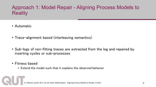
• Distinct sets of patterns can be used to explain the encountered difference
match B
lh = {}, rh = {}
m = {(e0,f0)A,(e1,f1)B}
rhide Cmatch C
lh = {}, rh = {f2:C}
m = {(e0,f0)A,(e1,f1)B}
lh = {}, rh = {}
m = {(e0,f0)A,(e1,f1)B,(e2,f2)C}
lh = {}, rh = {}
m = {(e0,f0)A}
match A
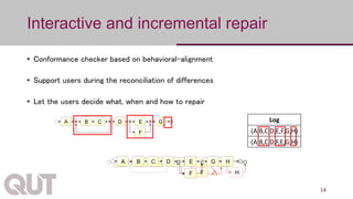
lh = {}, rh = {}
m = {}
match E
lh = {}, rh = {}
m = {(e0,f0)A,(e1,f1)B,(e2,f2)C,(e5,f4)E}
lh = {}, rh = {f2 : C, fx:E}
m = {(e0,f0)A, (e1,f1)B}
rhide E
• In the log, C is optional after {A,B}, whereas in the model
it is not
• In the log, task E does not occur after {A,B}
• In the log, task C does not occur after {A,B}
• In the log, task E does not occur after {A,B}
• In the log, the interval [C, E] is optional after {A,B},
whereas in the model it is not
30](https://image.slidesharecdn.com/coopis-171109133246/85/Incremental-and-Interactive-Process-Model-Repair-30-320.jpg)
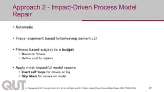
![Order of pattern detection
1. Patterns based on intervals
2. Patterns based on binary relations
3. Patterns based on a single task
i a b o
i o
c
ba
i a b o bc c
d
e
i a ob c
i a oec
TaskReloc: In the log, the interval [b,c] occurs after [i,a,o] instead of [i,a]
ConcConf: In the log, after i, Task a and Task b are concurrent, while in the model they
are mutually exclusive
i
a
o
b
i a o
b
i
a
o
b
i
a
o
b
i
a
o
b
TaskIns: In the log, Task b occurs after [i, a] and before o
New Process
i a b o
i a b o
i o
c
ba
i a b o b
i a o b
i a o
b](https://image.slidesharecdn.com/coopis-171109133246/85/Incremental-and-Interactive-Process-Model-Repair-31-320.jpg)


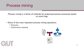
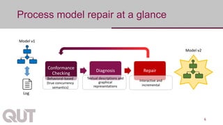
The document discusses process mining as a set of methods for analyzing business processes based on event logs, highlighting operations such as model discovery, conformance checking, and model repair. It presents two automatic approaches to process model repair: trace-alignment based and impact-driven. Additionally, the document emphasizes the importance of interactive and incremental model repair, allowing users to effectively reconcile differences between models and event logs.