The document summarizes methods for compressing precomputed radiance transfer (PRT) coefficients using spherical harmonics. It presents 4 methods with progressively higher compression ratios: Method 1 uses 9 bytes by removing a factor and scaling, Method 2 uses 6 bytes with a bit field allocation, Method 3 uses 6 bytes with a Lloyd-Max non-uniform quantizer, and Method 4 achieves 4 bytes with a different bit allocation. The methods are evaluated based on storage size, reconstruction quality, and rendering performance.

2. Practical Spherical Harmonics
Based PRT Methods
Manny Ko
Naughty Dog
Jerome Ko
UCSD / Bunkspeed

3. Outline
 Background ambient occlusion, HL2
 Spherical Harmonics theory
 Pre-processing
 PRT compression – 4 to 6 bytes per
sample
 Conclusion and game scene demo

4. Background
 Many variants of Precomputed
Radiance Transfer – self-shadow,
interreflections, diffuse vs. glossy
 Power of PRT best understood in the
context of ambient occlusion (AO)
and HL2 basis

5. Goals
 Diffuse self-shadowing for rigid
bodies (aka neighborhood transfer)
 Generalizes easily to interreflections
 Decouples visibility calculation from
lighting
 Pre-integrate surface variations

6. Ambient Occlusion
 Pioneered by ILM
 Accessibility shading

7. Ambient Occlusion

8. Ambient Occlusion Flavors
 Single scalar – cheap but no
directional response
 Bent Normal

9. Bent Normal: basic idea

10. Bent Normal
 Half3 + scalar AO = 7 bytes per
sample
 Give some directional variations but
it does not always work

11. Bent Normal: fail case

12. Bent Normal: next step
 Overcome the single direction,
single weight limitation

13. HL2 Basis
 Valve’s
“Radiosity
Normal
Mapping”
 3 RGB basis
vector per
sample

14. HL2 Samples

15. HL2 Strengths
 Successfully integrated GI with surface-
details
 Surface details respond to runtime lights
 1st attempt in games to use a ‘lighting
basis’
 Orthonormal basis
 Good for normal-maps

16. HL2 Weakness
 Lots of storage – 3 RGB maps per sample
plus UVs
 3 texture lookup + 3 dotp/ pixel after
rotating basis into tangent space. Shader
cost can be a problem.
 Incomplete coverage of the hemisphere,
3 directions not enough?

17. Key Ideas for PRT
 Visibilityis the key bottleneck since
it involves sampling the scene
 Take advantage of off-line compute
 Separate pre-integration of visibility
from that of incoming light
 Find a basis to store these functions

18. Key Ideas for PRT
 SH is a good starting point for a basis
 We do not trace rays using the GPU! Nor
do we take tons of samples inside the
pixel shader
 Better quality than AO or HL2 but more
efficient than later
 Work well for static scene + moving lights

19. Hovercraft from Warhawk

20. Demo
 Buddha – 1.08 m triangles
 33 fps on ATI X700
 250 fps on G8800 GTS
 Vertex shader only method
 Vertex buffer not optimized, could be
faster
 Dragon – 871k triangles
 40.7 fps on ATI X700

21. Implementation
Jerome Ko
UCSD / Bunkspeed

22. Outline
 Short introduction to SH (very
short!)
 Environment map projection
 PRT coefficient generation
 Runtime reconstruction in vertex
shader

23. Spherical Harmonics
 2D Fourier series on the sphere
 Represent 2D signals as scaled and
shifted Fourier basis.
 Perfect for spherical functions

24. Basis function Projection
Image courtesy of Real Time Rendering 3rd Edition

25. Spherical Harmonics Characteristics
 Orthonormal basis ->
 convolution as dot products
 simple projection
 Multi-resolution/band-limited,
related to Fourier decomposition
 Solid math foundation
 Stable rotation no wobbling lights
 Can add/subtract, lerp.

26. SH: bands (l,m)
 SH-order: order is the number of bands.
‘l’ is the order
 0th order: just a constant (DC) which is
your AO term
 1st order: 3 linear terms which is your
‘bent normal’ term
 2nd order: 5 terms – these give the extra
directional response we want
 In general (2l+1) terms

27. Spherical Harmonic
Functions

28. Spherical Harmonics - Issues
 Scary math!
 Looks difficult to implement
 Lots of coefficients, too much
storage?
 Difficult or time consuming to
generate?

29. Environment Map Projection
 First we need a light source
 Ravi R. introduced a technique to
light diffuse surfaces with distant
environment map illumination
 Code available on Ravi’s site, we
integrated it into our demo app

30. Environment Map Projection
 9 SH-compressed coefficients
 Instead of a large cubemap you
only need 27 numbers!
 Secret lies in the solid angle formula
 For each pixel evaluate the SH basis
then weighted it by the solid angle

31. Solid Angle
domega = 2*PI/width *
2*PI/height *
= (2*PI/width)*(2*PI/height)*sinc(theta);
sinc(theta);

32. Envmap Demo

33. PRT Coefficient Generation
 We have simplified the light source,
now we must also project the
visibility function using SH
 This gives us compact storage of
self-shadowing information
 Encodes the directional variations
more accurately than AO or HL2

34. Projecting Visibility Function

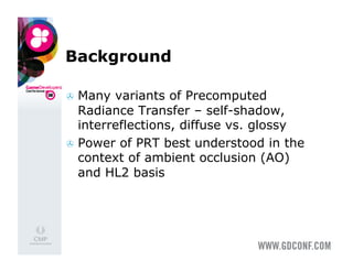
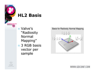
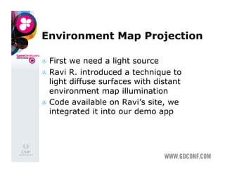
35. Projecting Visibility Function
for all samples {
stratified2D( u1, u2 ); //stratified random numbers
sampleHemisphere( shadowray, u1, u2, pdf[j] );
H = dot(shadowray.direction, vertexnormal);
if (H > 0) { //only use samples in upper hemisphere
if (!occludedByGeometry(shadowray)) {
for (int k = 0; k < bands; ++k) {
RGBCoeff& coeff = coeffentry[k];
//project onto SH basis
grayness = H * shcoeffs[j*bands + k];
grayness /= pdfs[j];
coeff += grayness; //sum up contribution
}
}
}
}

36. Projecting Visibility Function
 100-400 shadow rays per vertex are
sufficient
 Use your best acceleration structures
 Vertex normal is accounted for in
computation of H, thus no need for
normal in shader
 Full visibility function is preserved
 Group objects together in acceleration
structure to get inter-object shadowing

37. Runtime Reconstruction in
Vertex Shader
 The hard work has been done!
 Thanks to the orthogonality of SH
functions, reconstruction is reduced
to a simple dot product of 9 float3’s

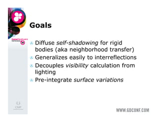
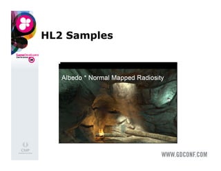
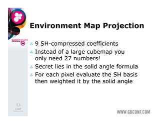
38. Runtime Reconstruction in
Vertex Shader
uniform vec3 Li[9];
attribute vec3 prt0;
attribute vec3 prt1;
attribute vec3 prt2;
color = Li[0]*(prt0.xxx) + Li[1]*
(prt0.yyy) + Li[2]*(prt0.zzz);
color += Li[3]*(prt1.xxx) + Li[4]*
(prt1.yyy) + Li[5]*(prt1.zzz);
color += Li[6]*(prt2.xxx) + Li[7]*
(prt2.yyy) + Li[8]*(prt2.zzz);

39. Comparison: With and
Without Self-Shadows

40. Comparison: With and
Without Self-Shadows

41. PRT in HyperDrive™

42. PRT Compression
Manny Ko
Naughty Dog

43. PRT Compression
 3rd order SH occupies 36 bytes per
sample
 Normals encoded as Lambertian response
during pre-processing
 World-space => no tangent space
needed.
 Bandwidth is key to GPU performance.
 PRT data size is key to pervasive usage in
game scenes.

44. Previous Work in PRT
Compression
 Sloan introduced CPCA
 Break mesh into small clusters
 PCA applied to each cluster to obtain a
reduced set of basis
 Fairly effective if the clusters are small but
that will add draw call overhead
 Hard to apply your vertex cache optimizer

45. Our PRT Compression
 M 1: 9 bytes using scale-bias
 M 2: 6 bytes (8; 6,6,6; 6,4,4,4,4)
 M 3: 6 bytes using Lloyd-Max
relaxation
 M 4: 4 bytes (5; 4,4,4 ;3,3,3,3,3)
 All very simple to implement

46. Scalar Quantizer and Scale-
Bias
 How to convert floats to bytes?
 Scan each sets of coefficients to get
range
 Ci = (Pi – Biasi) * Scalei ?
 We are dealing with a scalar
quantizer

47. Mid-rise vs. Mid-thread
Quantizer

48. Mid-rise Quantizer
 A 2 bit mid-rise quantizer has only 3
decision levels
 Advantage: can construct the DC-
level exactly. This can be critical in
some cases

49. Mid-thread Quantizer
 Even number of levels – e.g. 4
levels for a 2 bit code
 More accurate overall but cannot
reconstruct the DC-level
 For 4 bit codes we improved the
PSNR by ≈1db

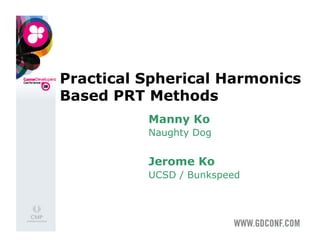
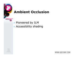
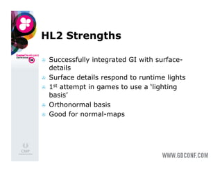
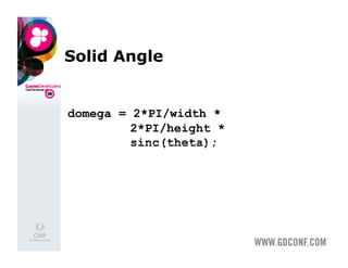
50. ScalarQuantizer
float half = (qkind == PRT::kMidRise) ?
0.5f : 0.f;
for (int i=0; i < nc; i++) {
float delta = scalars[i] – bias[i];
p[i] = delta * scales[i];
output[i] = floor(p[i] + half);
}

51. Method 1: 9 Bytes
 Use Mid-rise quantizer
 Remove 4PI factor from coefficients
 ¼ the memory and 2X improvement
in speed
 No visible quality lost, PSNR > 78db

52. Method 2: 48 Bits
 Method 1 takes us down to 9 bytes. Can
we do better?
 (8,6,6,6,6) (4,4,4,4) – bit fields
 Choice of bit allocation motivated by
• - Fourier theory => energy compaction
 - shader efficiency
 Cannot be optimal but try to be close

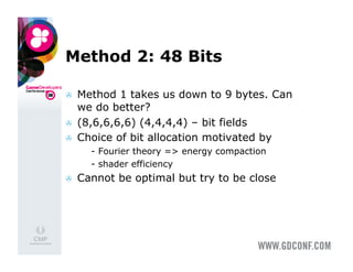
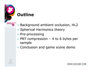
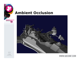
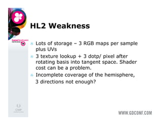
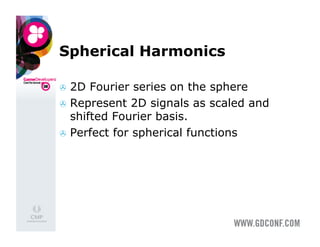
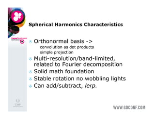
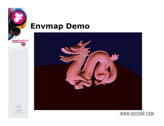
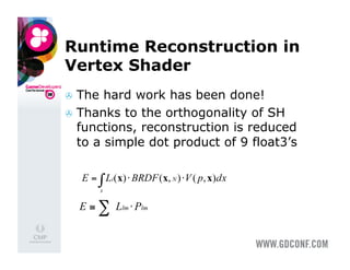
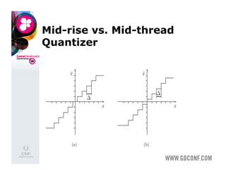
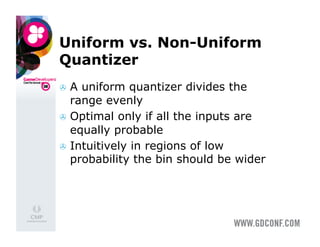
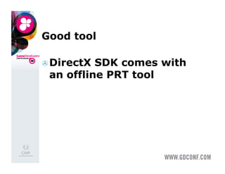
53. Square Norms by Band
 Energies by band
 [0]: 34.8%
 [1]: 17.1%
 [2]: 15.3%
 [3]: 17.1%
 85% of energies in 1st 4 bands

54. 1st word: 8,6,6,6,6
P0(b31..24),p1(23..18)..

55. Vertex Shader: Method 2
 Coefficients will straddle input
registers
 No bit operation in shaders – use
floating point ops to simulate
 Mul/div by power-of-2 for L/R shifts
 Fract and trunc() to isolate the 2
pieces. Add for ‘or’
 Tries to take advantage of SIMD

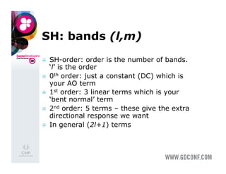
56. vertex shader
 // rshft(s[0], 1/4, 1/16, 1/64)
 p14 = prt0 * rshft;
 lhs3.yzw = fract(p14.yzw);
// lshft(0, 16.*4., 4.*16., 64.);
 lhs3 *= lshft;

 //p[0]:
 pp0 = p14.x + bias0;
 //p[1..4]:
 p14.xyz = (lhs3.xyz + floor(p14.yzw)) * scales.xyz
+ bias.xyz;
 p14.w = lhs3.w * scales.w + bias.w;

57. Comparison:M1 vs M2
184 fps 243 fps

58. Method 2: Demo and
Discussion
 Improved fps by ~17% compared with M1
 Reduced memory usage by 33%. More
with alignment restrictions
 Reduced the number of streams by 1 with
room to spare
 GFLOPS for modern GPU going up much
faster than bandwidth
 Looking for more mathops per byte?

59. Uniform vs. Non-Uniform
Quantizer
 A uniform quantizer divides the
range evenly
 Optimal only if all the inputs are
equally probable
 Intuitively in regions of low
probability the bin should be wider

60. Non-uniform quantizer
How can we design such a
set of bins?

61. Lloyd-Max Algorithm
 A version of k-means clustering algorithm
 Given a fixed number of bins iteratively
solves for an optimal set of bins
 Converges quickly
 Key is a probability distribution table (pdf)
 Applied to all 9 bands separatedly
 Details in ShaderX6

62. Lloyd-Max Iteration
 Given an initial set of bins tk..tk+1
 Find qk such that it is the centroid of tk..tk
+1
 Find tk so that it is the mid-point of qk..qk
+1
 Repeat for all the bins
 Check for convergence
 qks become the reconstruction levels.

63. Comparison:M2 vs M3

64. Quality increase for LM
 Improved the PSNR by 1.3
- 1.5db

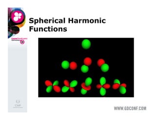
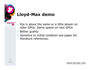
65. Shader for Lloyd-Max
 Almost the same as M2 since we are using
the same bit-allocation scheme
 Decoded bit-fields used to index a table of
reconstruction levels recon[]- the
centroids of the bins used in the quantizer
 can be constants or a small vertex texture
 Only used for 4 of the 2nd order terms

66. Lloyd-Max demo
 Fps is about the same or a little slower on
older GPUs. Same speed on new GPUs
 Better quality
 Sensitive to initial condition see paper for
literature references.

67. Game Scene Demo

68. Limitations
 Methods equally good for a
map based approach
 Distant Illumination
• Good for smaller objects
 For large objects either split them
or blend multiple Lis within
shader to avoid seams

69. Generalize to Interreflections
 Instead of sampling visibility gather
indirect illumination
 Use a photonmap or irradiance cache or
iteratively gather using visibility PRTs
 Use 3x48 or 3x32 bits per sample
 Or pack a 5,6,5 color with one of the 48
bit PRT methods.

70. Light Sources
 Not limited to environment maps
 Pre-integrate any kind of light
sources – preferable area lights or a
large collection of lights or use
probes
 Runtime methods to generate Lis
 Add or subtract lights easily – just
add/sub the Lis.
 Rotating lights is cheap

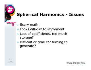
71. Normal maps
 Bake the normal variations and fine
surface details into the PRT
 Or use Peter-Pike’s [06] method

72. Good tool
 DirectX SDK comes with
an offline PRT tool

73. Conclusions
 Demonstrate how to implement all key
elements of a SH-based PRT shader
system
 Compact and efficient even for older GPUs
and no tangent space required
 Better than simple AO and bent-normal
 Smaller than bent-normal
 Groundwork for more GI effects

74. More on SH and PRT
 Peter-Pike’s talk Wed. 2:30pm
 Hao’s talk Thu. 4pm
 Yaohua’s talk Fri. 2:30pm

75. Contact Info
 Manny Ko – man961.great@gmail.com
 Jerome Ko – submatrix@gmail.com

76. Credits
 Matthias Zwicker for his guidance
and advising on the PRT research
 Ravi for all his help and generosity
 Peter-Pike S. for sharing his insights
 Incognito Studio for game assets
 Eric H. and Naty H. for figures
 Bunkspeed for screenshots
 All our friends

77. References
 [Green 07] “Surface Detail Maps with Soft
Self-Shadowing”, Siggraph 2007 Course.
 [Ko,Ko 08] “Practical Spherical Harmonics
based PRT Methods”, ShaderX6 2008.
 [McTaggart 04] “Half-Life 2 / Valve Source
Shading”, GDC 2004.
 [Mueller,Haines,Hoffman] Real Time
Rendering 3rd Edition.

78. References
 [Landis02] Production-Ready Global
Illumination, Siggraph 2002 Course.
 [Pharr 04] ”Ambient occlusion”,
GDC 2004.