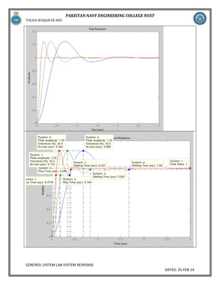
This document describes a lab experiment on system response for different order systems. It provides theory on transient and steady state responses. Tasks involve calculating transfer functions for different systems, finding pole-zero locations, and plotting step responses. Simulink is used to plot multiple step responses on a single graph for comparison. The objectives are to study effects of natural frequency, damping ratio, and pole locations on peak response, settling time, and rise time.

1. TALHA WAQAR EE-805
PAKISTAN NAVY ENGINEERING COLLEGE NUST
LAB # 3(A)
System Response
OBJECT:
To study the System response for different order systems, natural frequency and damping ratio, Peak
response, settling time, Rise time, steady state, using MATLAB commands and LTI Viewer.
THEORY:
Generally we have two types of responses, Steady State Response and Transient response such as rise
time, peak time, maximum overshoot, settling time etc.
n=[1 1];
Zero/pole/gain:
d=[2 4 6];
0.5 (s+1)
S1=tf(n,d)
--------------
size(S1) %no. of inputs and outputs.
(s^2 + 2s + 3)
pole(S1) % no.of poles .
pzmap(S1) %pole/zero map.
Eigenvalue
Damping
K=dcgain(S1)
-1.00e+000
1.73e+000
zpk(S1) % zero /pole/gain .
-1.00e+000 - 1.41e+000i
damp (S1) % damping coefficients.
wn =
[wn,z] = damp(S1) % naturalfrequency
1.41e+000i
5.77e-001
5.77e-001
1.73e+000
1.7321
step(S1) % assinging input for analysis
+
Freq. (rad/s)
1.7321
z=
Transfer function:
s+1
0.5774
0.5774
--------------2 s^2 + 4 s + 6
Transfer function with 1 outputs and 1 inputs.
ans =
-1.0000 + 1.4142i
-1.0000 - 1.4142i
K=
0.1667
CONTROL SYSTEM LAB SYSTEM RESPONSE
DATED: 25-FEB-14

2. TALHA WAQAR EE-805
PAKISTAN NAVY ENGINEERING COLLEGE NUST
zeta= [0.3 0.6 0.9 1.5]; % zeta funtion is assigned
with four different values.
for k=1:4; % k is assigned from 1-4 so as to run the
program four times in a loop.
num=[0 1 2]
den=[1 2*zeta(k) 1]; % den take out four different
values of zeta .
TF=tf(num,den)
step(TF)
hold on; % hold on restores the previous graphs.
end; % end represent the completion
num =
0
1
2
Transfer function:
s+2
--------------s^2 + 0.6 s + 1
num =
0 1
Transfer function:
s+2
--------------s^2 + 1.2 s + 1
num =
0
1
2
Transfer function:
s+2
--------------s^2 + 1.8 s + 1
num =
0
1
2
Transfer function:
s+2
------------s^2 + 3 s + 1
2
Exercise:
1. Given the transfer
function, G(s) = a/(s+a),
Evaluate settling time and
rise time for the following
values of a= 1, 2, 3, 4.
Also, plot the poles.
for k=1:4;
num=[k]
den=[1 k];
TF=tf(num,den)
step(TF)
hold on;
end
CONTROL SYSTEM LAB SYSTEM RESPONSE
DATED: 25-FEB-14

3. TALHA WAQAR EE-805
PAKISTAN NAVY ENGINEERING COLLEGE NUST
Lab task:
Task# 1:
CONTROL SYSTEM LAB SYSTEM RESPONSE
DATED: 25-FEB-14

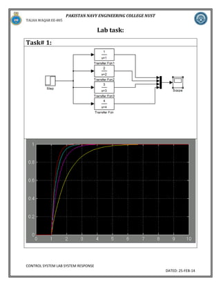
4. TALHA WAQAR EE-805
PAKISTAN NAVY ENGINEERING COLLEGE NUST
Task# 2a:
num=[25];
>> den=[1 4 25];
>> trans=tf(num,den);
>> step(trans);
>> zero(trans)
p=pole(t1)
p=
-2.0000 + 4.5826i2.0000 - 4.5826i
>> z=zero(t1)
z=
Empty matrix: 0by-1
>> y=pzmap (t1)
CONTROL SYSTEM LAB SYSTEM RESPONSE
DATED: 25-FEB-14

5. TALHA WAQAR EE-805
PAKISTAN NAVY ENGINEERING COLLEGE NUST
CONTROL SYSTEM LAB SYSTEM RESPONSE
DATED: 25-FEB-14

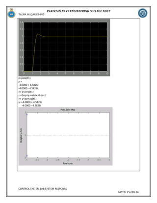
6. TALHA WAQAR EE-805
PAKISTAN NAVY ENGINEERING COLLEGE NUST
Task # 2b
>> trans=tf(num,den)
G(s)= b/s^2+as+b
Coefficent of damping I will represent with
C
poles= -C wn + -j wn sqrt 1-C^2
wn sqrt 1-C^2= 5*sqrt 1-a4^2=4.5826
C wn= 4 now wn=6.0828 & C=0.6575
Tp= .6949, Ts=1.0139, OS = .0645
a=7.89, b=36
Transfer function:
36
----------------s^2 + 7.86 s + 36
>> step(trans)
num=[36];
den=[1 7.86 36];
CONTROL SYSTEM LAB SYSTEM RESPONSE
DATED: 25-FEB-14

7. TALHA WAQAR EE-805
PAKISTAN NAVY ENGINEERING COLLEGE NUST
p=pole(t1)
p=
-4.0000 + 4.5826i
-4.0000 - 4.5826i
>> z=zero(t1)
z =Empty matrix: 0-by-1
>> y=pzmap(t1)
y =-4.0000 + 4.5826i
-4.0000 - 4.5826i
CONTROL SYSTEM LAB SYSTEM RESPONSE
DATED: 25-FEB-14

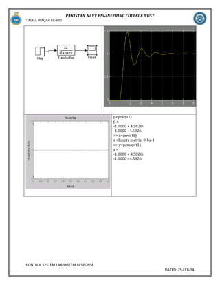
8. TALHA WAQAR EE-805
PAKISTAN NAVY ENGINEERING COLLEGE NUST
Task # 2c:
Calculate the values of a and b so that the imaginary part of the poles remains the same, but the real
part is decreased ½ time over that of (a), and repeat the 2(a).
num=[22];
>> den=[1 2 22];
>> trans=tf(num,den);
>> step(trans)
>>zero(trans)
ans =
Empty matrix: 0-by-1
CONTROL SYSTEM LAB SYSTEM RESPONSE
DATED: 25-FEB-14

9. TALHA WAQAR EE-805
PAKISTAN NAVY ENGINEERING COLLEGE NUST
p=pole(t1)
p=
-1.0000 + 4.5826i
-1.0000 - 4.5826i
>> z=zero(t1)
z =Empty matrix: 0-by-1
>> y=pzmap(t1)
y=
-1.0000 + 4.5826i
-1.0000 - 4.5826i
CONTROL SYSTEM LAB SYSTEM RESPONSE
DATED: 25-FEB-14

10. TALHA WAQAR EE-805
PAKISTAN NAVY ENGINEERING COLLEGE NUST
Task # 3a:
For the system of prelab 2(a) calculate the values of a and b so that the realpart of the poles remains
the same but the imaginary part is increased 2times ove that of prelab 2(a) and repeat prelab 2(a)
A=4,b=88
num=[88];
>> den=[1 4 88];
>> trans=tf(num,den);
>> step(trans)
CONTROL SYSTEM LAB SYSTEM RESPONSE
DATED: 25-FEB-14

11. TALHA WAQAR EE-805
PAKISTAN NAVY ENGINEERING COLLEGE NUST
p=pole(t1)
p=
-2.0000 + 9.1652i
-2.0000 - 9.1652i
z=zero(t1)
z=
Empty matrix: 0-by-1
>> y=pzmap(t1)
y=
-2.0000 + 9.1652i
-2.0000 - 9.1652i
Task # 3b
CONTROL SYSTEM LAB SYSTEM RESPONSE
DATED: 25-FEB-14

12. TALHA WAQAR EE-805
PAKISTAN NAVY ENGINEERING COLLEGE NUST
For the system of prelab 2(a) calculate the values of a and b so that the realpart of the poles remains
the same but the imaginary part is increased 4times over that of prelab 2(a) and repeat prelab 2(a)
A=4,b=340
num=[340];
>> den=[1 4 340];
>> trans=tf(num,den)
Transfer function:
340
--------------s^2 + 4 s + 340
>> step(trans)
CONTROL SYSTEM LAB SYSTEM RESPONSE
DATED: 25-FEB-14

13. TALHA WAQAR EE-805
PAKISTAN NAVY ENGINEERING COLLEGE NUST
p=pole(t1)
p=
-2.0000 +18.3303i
-2.0000 -18.3303i
>> z=zero(t1)
z=
Empty matrix: 0-by-1
>> y=pzmap(t1)
y=
-2.0000 +18.3303i
-2.0000 -18.3303i
CONTROL SYSTEM LAB SYSTEM RESPONSE
DATED: 25-FEB-14

14. TALHA WAQAR EE-805
PAKISTAN NAVY ENGINEERING COLLEGE NUST
Task # 4a
For the system of 2(a), calculate the values of a and b so that the damping ratio remains the same, but
the natural frequency is increased 2 times over that of 2(a), and repeat 2(a).
num=[100];
>> den=[1 8 100];
>> trans=tf(num,den)
Transfer function:
100
--------------s^2 + 8 s + 100
>> step(trans)
CONTROL SYSTEM LAB SYSTEM RESPONSE
DATED: 25-FEB-14

15. TALHA WAQAR EE-805
PAKISTAN NAVY ENGINEERING COLLEGE NUST
Task # 4b:
CONTROL SYSTEM LAB SYSTEM RESPONSE
DATED: 25-FEB-14

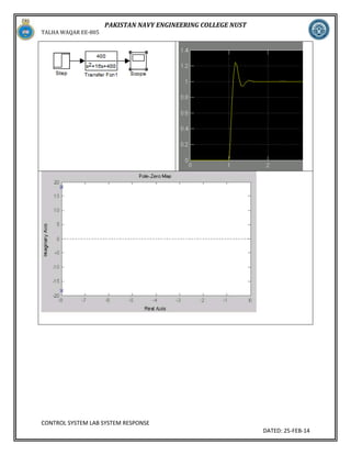
16. TALHA WAQAR EE-805
PAKISTAN NAVY ENGINEERING COLLEGE NUST
For the system of 2(a), calculate the values of a and b so that the damping ratio remains the same, but
the natural frequency is increased 4 times over that of 2(a), and repeat 2(a).
eeta=0.4
>> omega=20
omega=20
>> b=omega*omegab =400
>> a=2*eeta*omegaa =16
>> num=[b]num=400
>> den=[ 1 a b]
den =
1 16 400
>> t=tf([num],[den])
Transfer function:
400
s^2 + 16 s + 400
CONTROL SYSTEM LAB SYSTEM RESPONSE
DATED: 25-FEB-14

17. TALHA WAQAR EE-805
PAKISTAN NAVY ENGINEERING COLLEGE NUST
CONTROL SYSTEM LAB SYSTEM RESPONSE
DATED: 25-FEB-14

18. TALHA WAQAR EE-805
PAKISTAN NAVY ENGINEERING COLLEGE NUST
Exercise:
Using Simulink, set up the systems of Q 2. Using the Simulink LTI Viewer, plot the step response of each
of the 3 transfer functions on a single graph.
a=tf([25],[1 4 25]);
>> b=tf([37],[1 8 37]);
>> c=tf([22],[1 2 22]);
>> step(a,b,c)
CONTROL SYSTEM LAB SYSTEM RESPONSE
DATED: 25-FEB-14

19. TALHA WAQAR EE-805
PAKISTAN NAVY ENGINEERING COLLEGE NUST
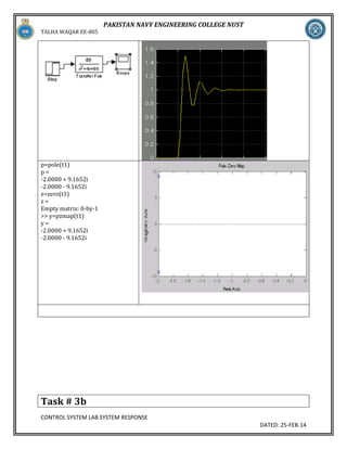
task # 3:
Using Simulink, set up the systems of Q2(a) and Q3. Using the Simulink LTI Viewer, plot the step
response of each of the 3 transfer functions on a single graph.
c=tf([25],[1 4 25]);
>> b=tf([88],[1 4 88]);
>> a=tf([340],[1 4 340]);
>> step(a,b,c)
CONTROL SYSTEM LAB SYSTEM RESPONSE
DATED: 25-FEB-14

20. TALHA WAQAR EE-805
PAKISTAN NAVY ENGINEERING COLLEGE NUST
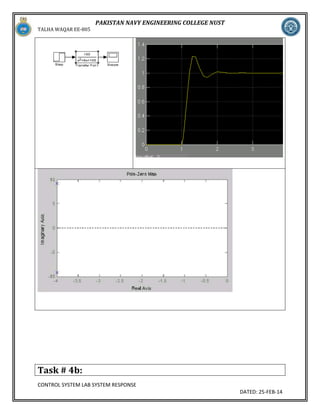
Task # 4:
Using Simulink, set up the systems of Q 2(a) and Q 4. Using the Simulink LTI Viewer, plot the step
response of each of the 3 transfer functions on a single graph.
a=tf([25],[1 4 25]);
>> b=tf([100],[1 8 100]);
>> c=tf([400],[1 16 400]);
>> step(a,b,c)
CONTROL SYSTEM LAB SYSTEM RESPONSE
DATED: 25-FEB-14

21. TALHA WAQAR EE-805
PAKISTAN NAVY ENGINEERING COLLEGE NUST
CONTROL SYSTEM LAB SYSTEM RESPONSE
DATED: 25-FEB-14