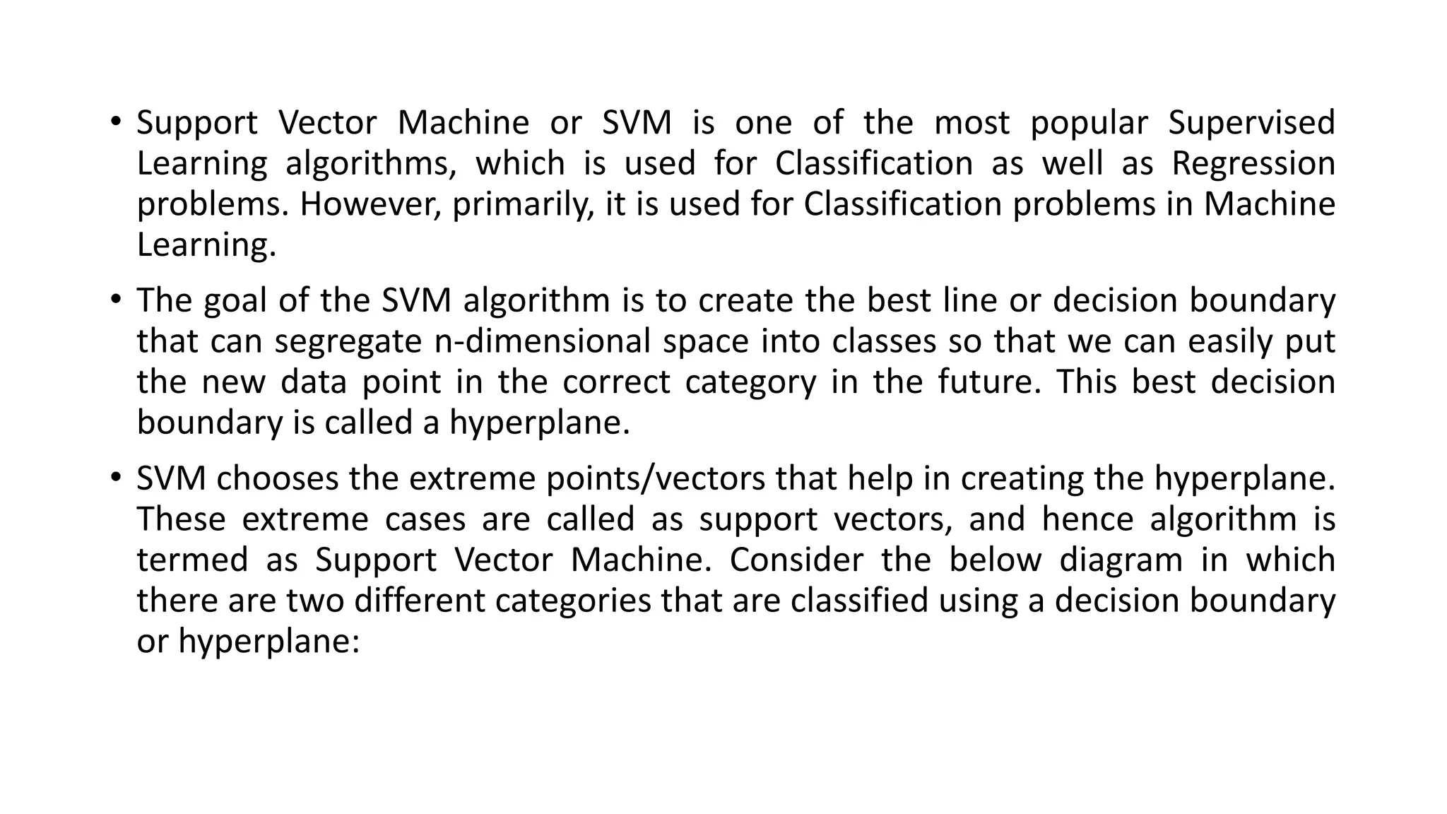
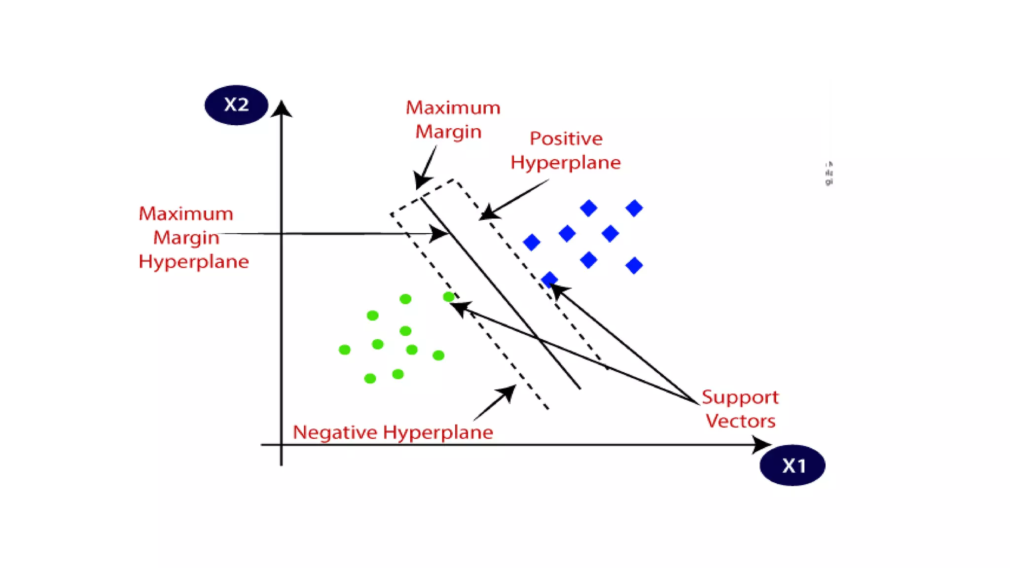
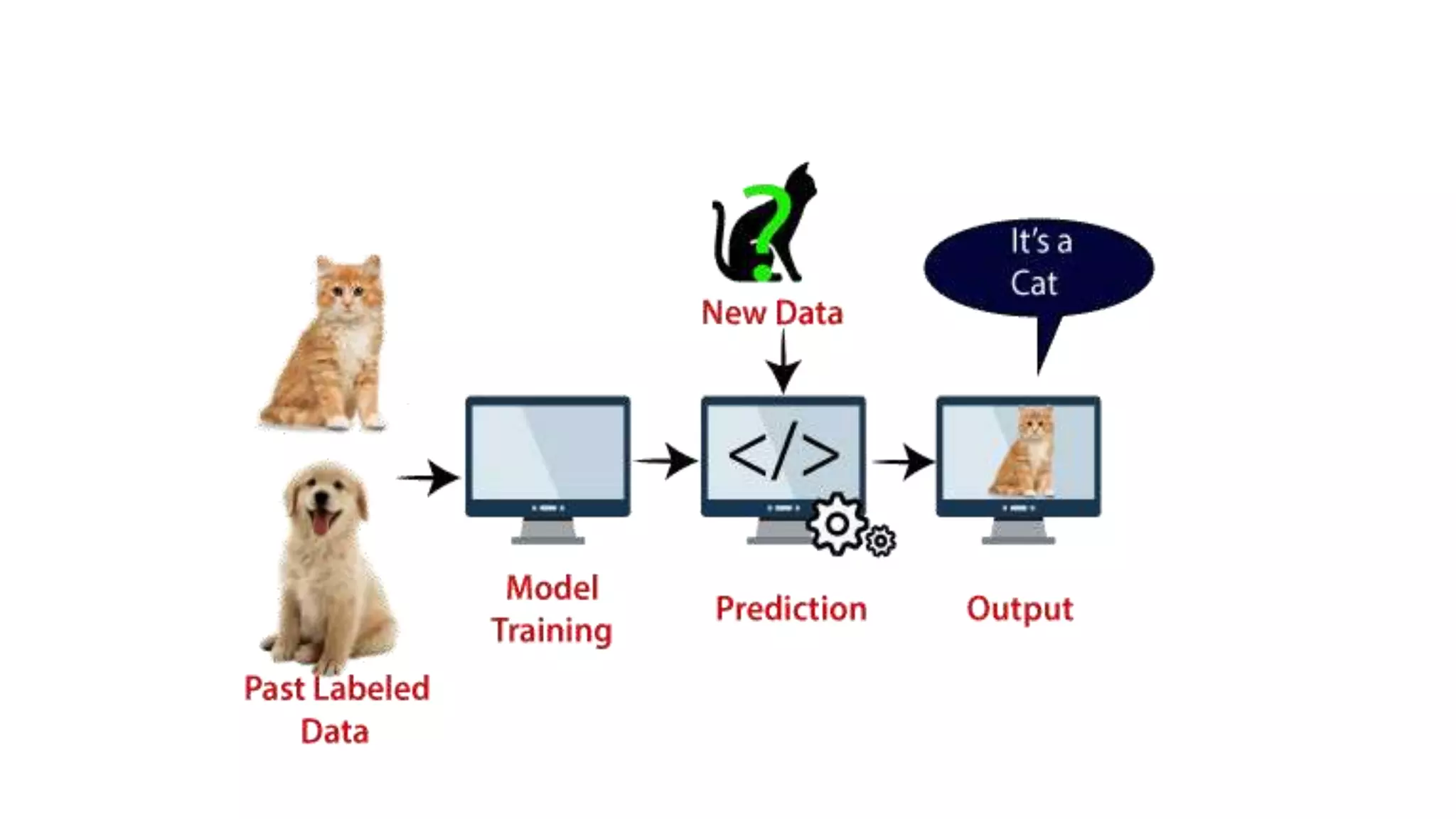
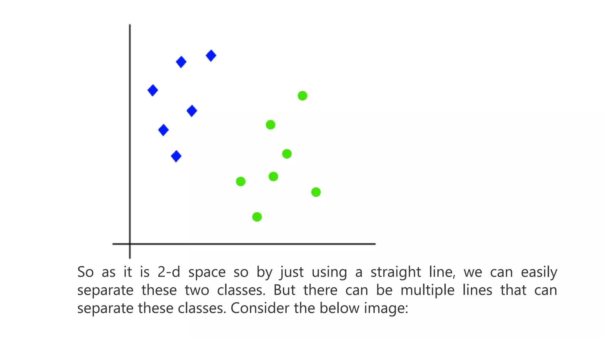
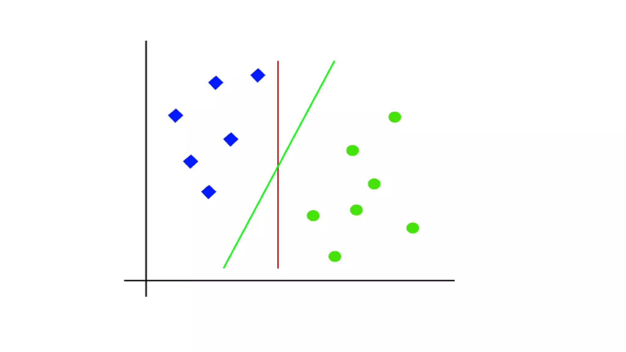
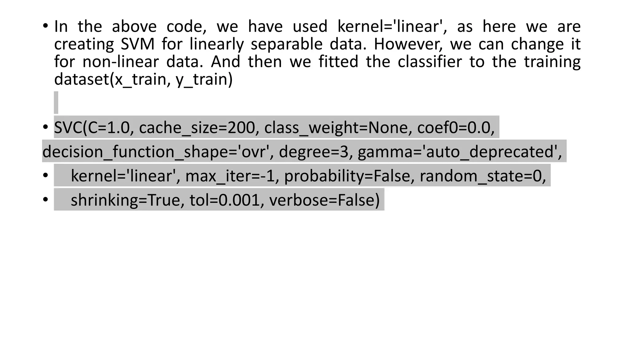
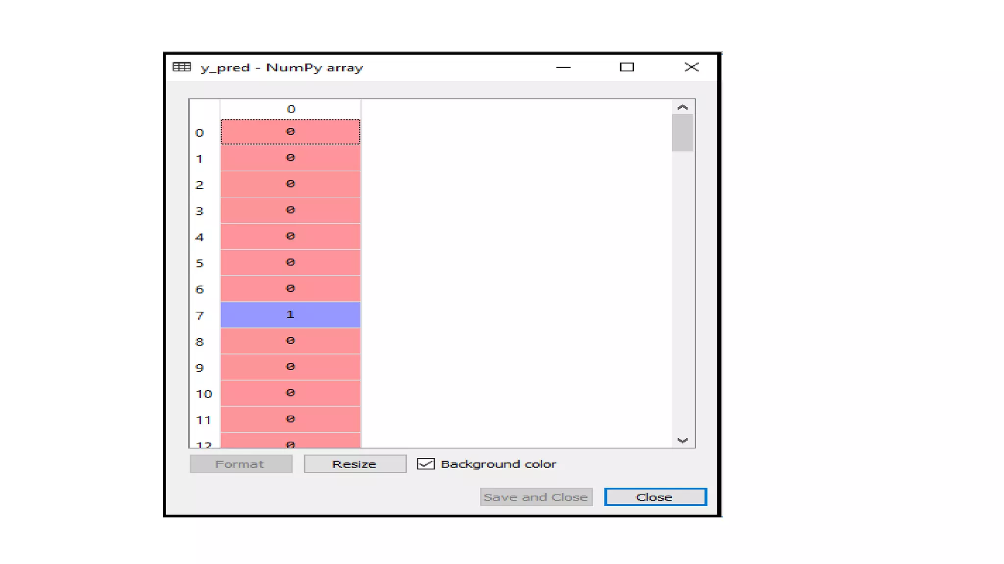
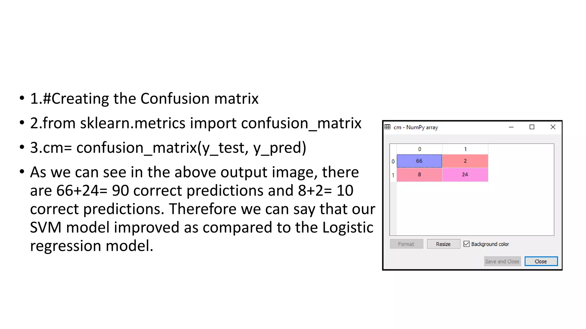
The document discusses the Support Vector Machine (SVM) algorithm. It begins by explaining that SVM is a supervised learning algorithm used for classification and regression. It then describes how SVM finds the optimal decision boundary or "hyperplane" that separates cases in different categories by the maximum margin. The extreme cases that define this margin are called "support vectors." The document provides an example of using SVM to classify images as cats or dogs. It explains the differences between linear and non-linear SVM models and provides code to implement SVM in Python.

1. Support Vector Machine
Algorithm

2. • Support Vector Machine or SVM is one of the most popular Supervised
Learning algorithms, which is used for Classification as well as Regression
problems. However, primarily, it is used for Classification problems in Machine
Learning.
• The goal of the SVM algorithm is to create the best line or decision boundary
that can segregate n-dimensional space into classes so that we can easily put
the new data point in the correct category in the future. This best decision
boundary is called a hyperplane.
• SVM chooses the extreme points/vectors that help in creating the hyperplane.
These extreme cases are called as support vectors, and hence algorithm is
termed as Support Vector Machine. Consider the below diagram in which
there are two different categories that are classified using a decision boundary
or hyperplane:

4. • Example: SVM can be understood with the example that we have used in
the KNN classifier. Suppose we see a strange cat that also has some
features of dogs, so if we want a model that can accurately identify
whether it is a cat or dog, so such a model can be created by using the
SVM algorithm. We will first train our model with lots of images of cats
and dogs so that it can learn about different features of cats and dogs,
and then we test it with this strange creature. So as support vector
creates a decision boundary between these two data (cat and dog) and
choose extreme cases (support vectors), it will see the extreme case of
cat and dog. On the basis of the support vectors, it will classify it as a
cat. Consider the below diagram:

6. • SVM algorithm can be used for Face detection, image classification, text
categorization, etc.
• Types of SVM
• SVM can be of two types:
• Linear SVM: Linear SVM is used for linearly separable data, which
means if a dataset can be classified into two classes by using a single
straight line, then such data is termed as linearly separable data, and
classifier is used called as Linear SVM classifier.
• Non-linear SVM: Non-Linear SVM is used for non-linearly separated
data, which means if a dataset cannot be classified by using a straight
line, then such data is termed as non-linear data and classifier used is
called as Non-linear SVM classifier.

7. Hyperplane and Support Vectors in the SVM
algorithm:
• Hyperplane: There can be multiple lines/decision boundaries to segregate the classes in
n-dimensional space, but we need to find out the best decision boundary that helps to
classify the data points. This best boundary is known as the hyperplane of SVM.
• The dimensions of the hyperplane depend on the features present in the dataset, which
means if there are 2 features (as shown in image), then hyperplane will be a straight line.
And if there are 3 features, then hyperplane will be a 2-dimension plane.
• We always create a hyperplane that has a maximum margin, which means the maximum
distance between the data points.
• Support Vectors:
• The data points or vectors that are the closest to the hyperplane and which affect the
position of the hyperplane are termed as Support Vector. Since these vectors support the
hyperplane, hence called a Support vector.

8. How does SVM works?
• Linear SVM:
• The working of the SVM algorithm can be understood by using an
example. Suppose we have a dataset that has two tags (green and
blue), and the dataset has two features x1 and x2. We want a
classifier that can classify the pair(x1, x2) of coordinates in either
green or blue. Consider the below image

9. So as it is 2-d space so by just using a straight line, we can easily
separate these two classes. But there can be multiple lines that can
separate these classes. Consider the below image:

11. • Hence, the SVM algorithm helps to find the best line or decision
boundary; this best boundary or region is called as a hyperplane. SVM
algorithm finds the closest point of the lines from both the classes.
These points are called support vectors. The distance between the
vectors and the hyperplane is called as margin. And the goal of SVM is
to maximize this margin. The hyperplane with maximum margin is
called the optimal hyperplane.

12. Python Implementation of Support Vector
Machine
• Now we will implement the SVM algorithm using Python. Here we
will use the same dataset user_data, which we have used in Logistic
regression and KNN classification.
• Data Pre-processing step
• Till the Data pre-processing step, the code will remain the same.
Below is the code:

13. #Data Pre-processing Step
# importing libraries
#import numpy as nm
#import matplotlib.pyplot as mtp
#import pandas as pd
#importing datasets
data_set= pd.read_csv('user_data.csv')

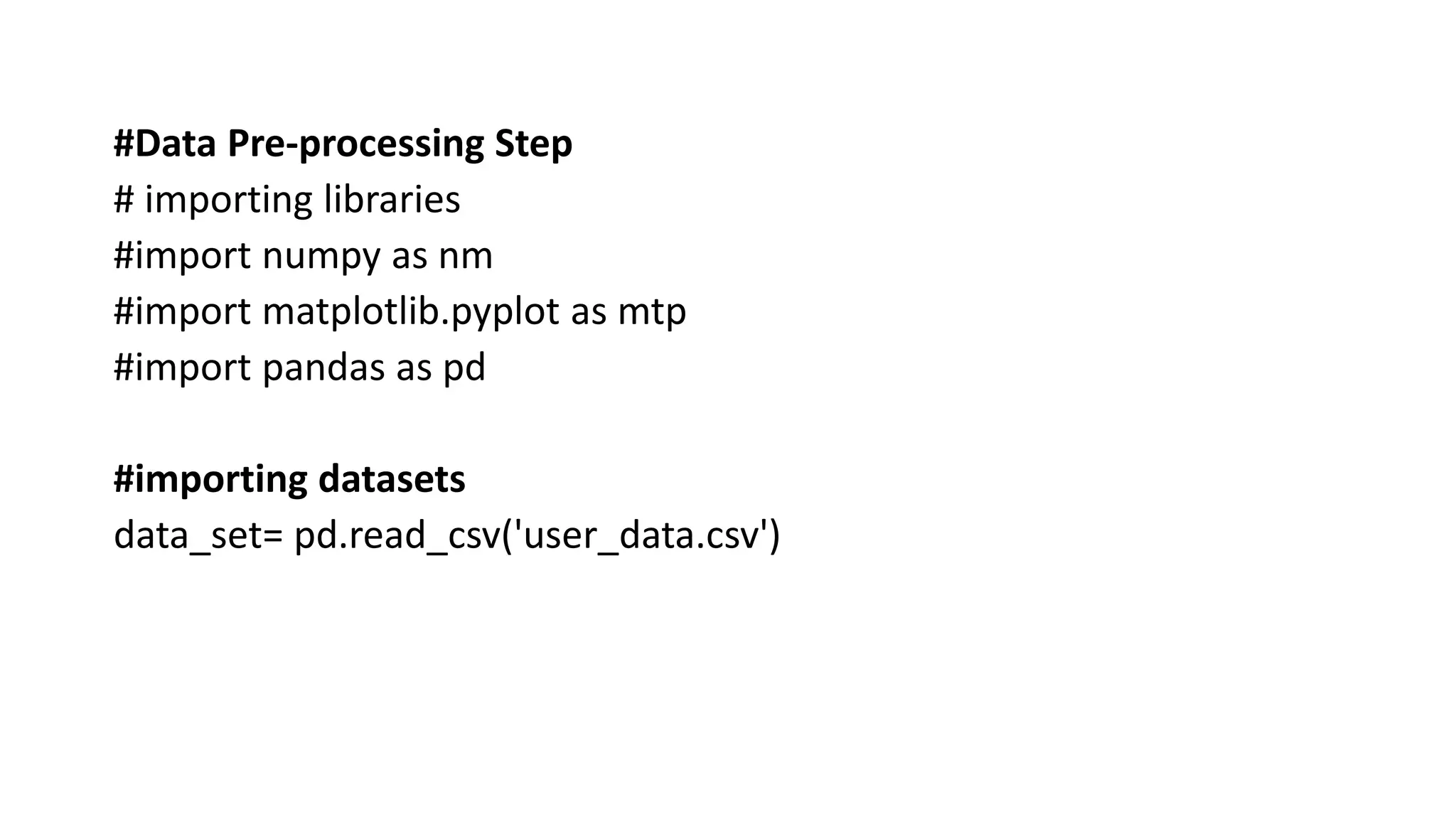
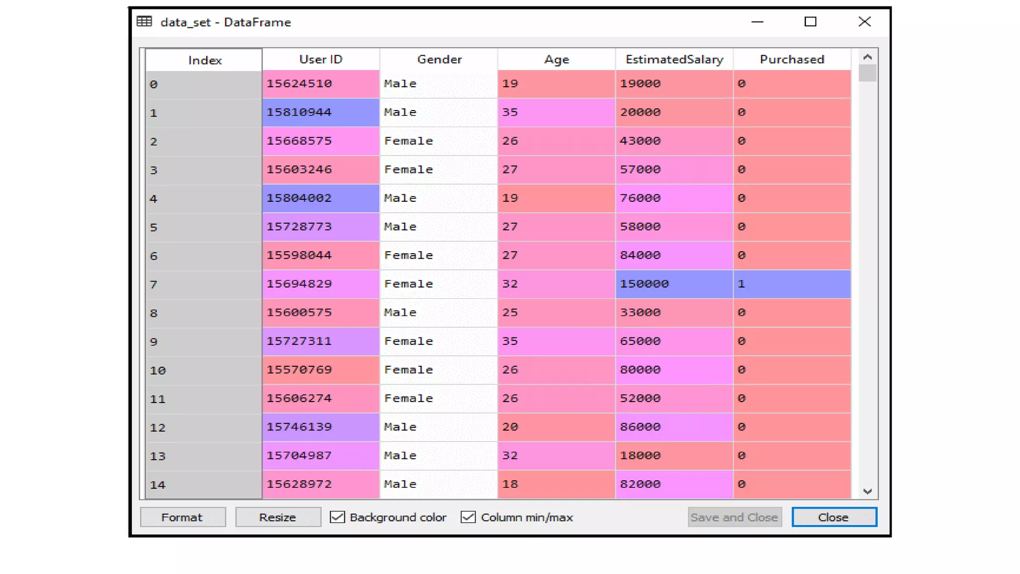
14. #Extracting Independent and dependent Variable
x= data_set.iloc[:, [2,3]].values
y= data_set.iloc[:, 4].values
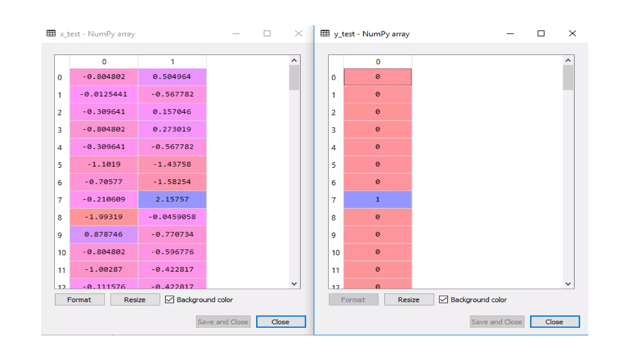
# Splitting the dataset into training and test set.
from sklearn.model_selection import train_test_split
x_train, x_test, y_train, y_test= train_test_split(x, y, test_size= 0.25, random_state=0)
#feature Scaling
from sklearn.preprocessing import StandardScaler
st_x= StandardScaler()
x_train= st_x.fit_transform(x_train)
x_test= st_x.transform(x_test)

17. • Fitting the SVM classifier to the training set:
• Now the training set will be fitted to the SVM classifier. To create the
SVM classifier, we will import SVC class from Sklearn.svm library.
Below is the code for it:
• 1.from sklearn.svm import SVC # "Support vector classifier"
• 2.classifier = SVC(kernel='linear', random_state=0)
• 3.classifier.fit(x_train, y_train)

18. • In the above code, we have used kernel='linear', as here we are
creating SVM for linearly separable data. However, we can change it
for non-linear data. And then we fitted the classifier to the training
dataset(x_train, y_train)
• SVC(C=1.0, cache_size=200, class_weight=None, coef0=0.0,
decision_function_shape='ovr', degree=3, gamma='auto_deprecated',
• kernel='linear', max_iter=-1, probability=False, random_state=0,
• shrinking=True, tol=0.001, verbose=False)

19. • The model performance can be altered by changing the value
of C(Regularization factor), gamma, and kernel.
• Predicting the test set result:
• Now, we will predict the output for test set. For this, we will create a
new vector y_pred. Below is the code for it:
• #Predicting the test set result
• y_pred= classifier.predict(x_test)
• After getting the y_pred vector, we can compare the result
of y_pred and y_test to check the difference between the actual value
and predicted value.
• Output: Below is the output for the prediction of the test set:

21. Creating the confusion matrix:
• Now we will see the performance of the SVM classifier that how
many incorrect predictions are there as compared to the Logistic
regression classifier. To create the confusion matrix, we need to
import the confusion_matrix function of the sklearn library. After
importing the function, we will call it using a new variable cm. The
function takes two parameters, mainly y_true( the actual values)
and y_pred (the targeted value return by the classifier). Below is the
code for it:

22. • 1.#Creating the Confusion matrix
• 2.from sklearn.metrics import confusion_matrix
• 3.cm= confusion_matrix(y_test, y_pred)
• As we can see in the above output image, there
are 66+24= 90 correct predictions and 8+2= 10
correct predictions. Therefore we can say that our
SVM model improved as compared to the Logistic
regression model.