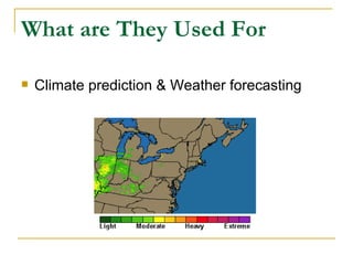
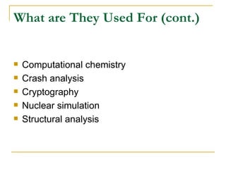
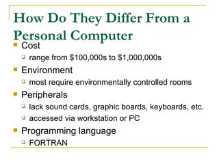
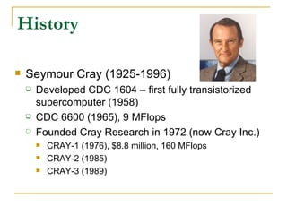
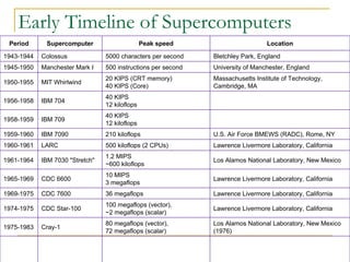
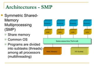
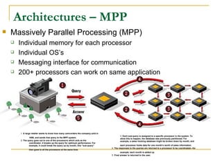
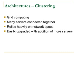
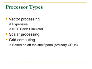
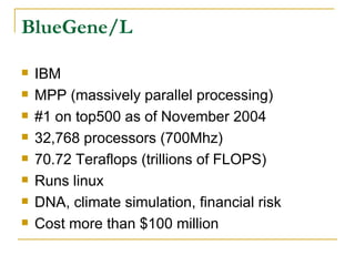
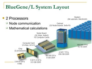
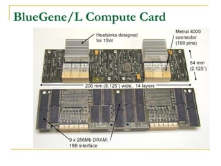
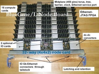
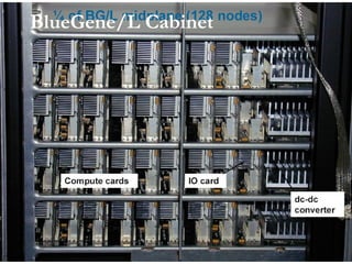
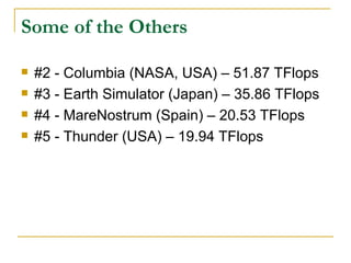
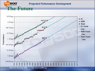
This document provides an overview of supercomputers including their uses, history, architectures, and key systems. Supercomputers are the most powerful and expensive computers available designed to solve complex problems quickly. They are used for tasks like weather forecasting, nuclear simulation, and cryptography. They differ from personal computers in cost, environment, programming languages, and lack of common peripherals. Major early systems included the CDC 6600 and Cray-1. Current systems use clustering, symmetric multiprocessing, or massively parallel processing architectures. The top systems include BlueGene/L, Columbia, and Earth Simulator.

1. Overview of
Supercomputers
Presented by:
Mehmet Demir
20090694
ENG-102

2. Table of Contents
 Introduction
 What are They Used For
 How Do They Differ From a Personal Computer?
 Where Are They Now
 Main Parts of Supercomputers
 Processor Types
 Conclusion
 References

3. Supercomputers
 The category of computers that includes the
fastest and most powerful (most expensive)
ones available at any given time.
 Designed to solve complex mathematical
equations and computational problems very
quickly.

4. What are They Used For
 Climate prediction & Weather forecasting

5. What are They Used For (cont.)
 Computational chemistry
 Crash analysis
 Cryptography
 Nuclear simulation
 Structural analysis

6. How Do They Differ From a
Personal Computer
 Cost
 range from $100,000s to $1,000,000s
 Environment
 most require environmentally controlled rooms
 Peripherals
 lack sound cards, graphic boards, keyboards, etc.
 accessed via workstation or PC
 Programming language
 FORTRAN

7. History
 Seymour Cray (1925-1996)
 Developed CDC 1604 – first fully transistorized
supercomputer (1958)
 CDC 6600 (1965), 9 MFlops
 Founded Cray Research in 1972 (now Cray Inc.)
 CRAY-1 (1976), $8.8 million, 160 MFlops
 CRAY-2 (1985)
 CRAY-3 (1989)

8. Early Timeline of Supercomputers
Period Supercomputer Peak speed Location
1943-1944 Colossus 5000 characters per second Bletchley Park, England
1945-1950 Manchester Mark I 500 instructions per second University of Manchester, England
20 KIPS (CRT memory) Massachusetts Institute of Technology,
1950-1955 MIT Whirlwind
40 KIPS (Core) Cambridge, MA
40 KIPS
1956-1958 IBM 704
12 kiloflops
40 KIPS
1958-1959 IBM 709
12 kiloflops
1959-1960 IBM 7090 210 kiloflops U.S. Air Force BMEWS (RADC), Rome, NY
1960-1961 LARC 500 kiloflops (2 CPUs) Lawrence Livermore Laboratory, California
1.2 MIPS
1961-1964 IBM 7030 "Stretch" Los Alamos National Laboratory, New Mexico
~600 kiloflops
10 MIPS
1965-1969 CDC 6600 Lawrence Livermore Laboratory, California
3 megaflops
1969-1975 CDC 7600 36 megaflops Lawrence Livermore Laboratory, California
100 megaflops (vector),
1974-1975 CDC Star-100 Lawrence Livermore Laboratory, California
~2 megaflops (scalar)
80 megaflops (vector), Los Alamos National Laboratory, New Mexico
1975-1983 Cray-1
72 megaflops (scalar) (1976)

9. Where Are They Now
 www.top500.org
 List released twice a year
 Scores based on Linpack benchmark
 Solve dense system of linear equations
 Speed measured in floating point operations
per second (FLOPS)

10. Architectures - SMP
 Symmetric Shared-
Memory
Multiprocessing
(SMP)
 Share memory
 Common OS
 Programs are divided
into subtasks (threads)
among all processors
(multithreading)

11. Architectures – MPP
 Massively Parallel Processing (MPP)
 Individual memory for each processor
 Individual OS’s
 Messaging interface for communication
 200+ processors can work on same application
1. A large retailer wants to know how many camcorders the company sold in
3. Each sub-query is assigned to a specific processor in the system. To
1998, and sends that query to the MPP system. allow this to happen, the database was previously partitioned. For
2. The query goes out to one of the processors which acts as the example, a sales tracking database might be broken down by month, and
coordinator, it breaks up the query for optimum performance. For
example, it could break the query up by month; this “sub-query” each processor holds data for one month’s worth of sales information.
4. The responses to the queries are returned to a processor to be coordinated—for
then goes to all the processors at the same time.
example, each month is added up
5. Final answer is returned to the user.

12. Architectures – Clustering
 Grid computing
 Many servers connected together
 Relies heavily on network speed
 Easily upgraded with addition of more servers

13. Processor Types
 Vector processing
 Expensive
 NEC Earth Simulator
 Scalar processing
 Grid computing
 Based on off the shelf parts (ordinary CPUs)

14. BlueGene/L
 IBM
 MPP (massively parallel processing)
 #1 on top500 as of November 2004
 32,768 processors (700Mhz)
 70.72 Teraflops (trillions of FLOPS)
 Runs linux
 DNA, climate simulation, financial risk
 Cost more than $100 million

15. BlueGene/L System Layout
 2 Processors
 Node communication
 Mathematical calculations

16. BlueGene/L Compute Card

17. BlueGene/L Node Board

18. BlueGene/L Cabinet

19. Some of the Others
 #2 - Columbia (NASA, USA) – 51.87 TFlops
 #3 - Earth Simulator (Japan) – 35.86 TFlops
 #4 - MareNostrum (Spain) – 20.53 TFlops
 #5 - Thunder (USA) – 19.94 TFlops

20. The Future

21. References
 http://www.top500.org/
 http://www.pcquest.com/content/Supercomputer/102051
004.asp
 http://news.com.com/2100-1008_3-1000421.html?
tag=fd_lede2_hed
 http://www.research.ibm.com/bluegene/index.html
 http://www.llnl.gov/asci/platforms/bluegene/papers/2hard
ware_overview.pdf
 http://www.hpce.nec.com/451+M5f7cd421b8e.0.html
 http://www.cray.com/about_cray/history.html
 http://www.serc.iisc.ernet.in/~govind/243/L7-PA-Intro.pdf
 http://www.computerworld.com/hardwaretopic
s/hardware/server/story/0,10801,43504,00.ht
ml