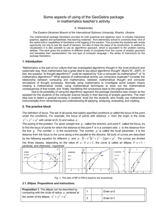
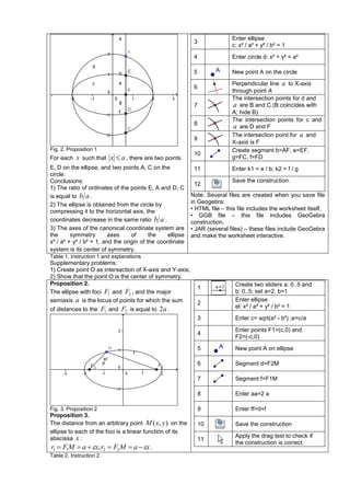
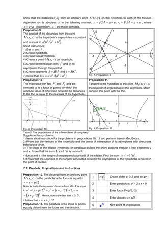
The document discusses using the GeoGebra mathematical software package in mathematics teaching. It presents 14 propositions about ellipses, hyperbolas, and parabolas. Students used GeoGebra's interactive features to construct the curves as loci of points and solve problems of varying complexity based on the propositions. This reinforced their understanding of concepts from the "Second-Order Curves" course material from sources like textbooks and papers.

1. Some aspects of using of the GeoGebra package
in mathematics teacher’s activity
A. Stolyarevska
The Eastern-Ukrainian Branch of the International Solomon University, Kharkiv, Ukraine
The mathematical package GeoGebra provides for both graphical and algebraic input. It includes interactive
graphics, algebra and spreadsheet, free learning materials - from elementary school to university level. One of
the useful built-in capabilities of GeoGebra is the logging of the solution. This provides the students with ample
opportunity not only to see the result of decision, but also to trace the steps of its construction. In addition to
visualization it is also possible to use an algorithmic approach, which is equivalent to the problem solving
abilities. This work gives the problems of different levels of complexity from the course of analytic geometry
and translates their representation into one type of computer language – the series of instructions for the
package GeoGebra.
1. Introduction
“Mathematics is the part of our culture that has investigated algorithmic thought in the most profound and
systematic way. Now mathematics has a great deal to say about algorithmic thought” (Byers W., 2007). In
fact, the question “Is thought algorithmic?” could be replaced by “Can a computer do mathematics?” or “Is
mathematics algorithmic?” What aspects of mathematical activity can computers duplicate? Consider the
relationship between computing and mathematics, between mathematical thought and computer
simulations of thought processes. Normally using mathematics to investigate some subject means
creating a mathematical model, using mathematical techniques to draw out the mathematical
consequences of that model, and, finally, translating the conclusions back to the original situation.
Due to its possibility of using the algorithmic approach the package GeoGebra was chosen as the
assistant for the students of the computer science faculty in their learning of analytic geometry. The main
idea was to detect a gradual increase in students’ level (for the students, who mostly use mathematics
instrumentally) from remembering and understanding till applying, analyzing, evaluating, and creating.
2. The practice block
The definition of locus. The set of all points that satisfy specified conditions is called the locus of the point
under the conditions. For example, the locus of points with distance a from the origin is the circle
222
ayx  with center at (0, 0) and radius a .
The posing of the problem. For given straight line g , called the directrix, and point F, called the focus, try
to find the locus of points for which the distance to the point F is in a constant ratio  to the distance from
the line g . The number  is the eccentricity. The number p is called the focal parameter, it is the
distance from the focus to the curve along a line parallel to the directrix. All sorts of curves are described
by the following equation for different  and p :   2222
21 ppxyx   . The curves are divided
into three classes, depending on the value of  : if 1 , the curve is called an ellipse, if 1 -
parabola, and otherwise - hyperbola.
Fig. 1. The ratio of MF to KM is equal to the eccentricity
2.1. Ellipse. Propositions and instructions
Proposition 1. The ellipse can be described by
comparing with the circle of radius a centered at
the center of the ellipse:
222
ayx  .
1 Enter a=2
2 Enter b=1

2. Fig. 2. Proposition 1
For each x such that ax  , there are two points
E, D on the ellipse, and two points A, C on the
circle.
Conclusions:
1) The ratio of ordinates of the points E, A and D, C
is equal to ab .
2) The ellipse is obtained from the circle by
compressing it to the horizontal axis, the
coordinates decrease in the same ratio ab .
3) The axes of the canonical coordinate system are
the symmetry axes of the ellipse
x² / a² + y² / b² = 1, and the origin of the coordinate
system is its center of symmetry.
3
Enter ellipse
c: x² / a² + y² / b² = 1
4 Enter circle d: x² + y² = a²
5 New point A on the circle
6
Perpendicular line a to X-axis
through point A
7
The intersection points for d and
a are B and C (B coincides with
A; hide B)
8
The intersection points for c and
a are D and F
9
The intersection point for a and
X-axis is F
10
Create segment b=AF, e=EF,
g=FC, f=FD
11 Enter k1 = e / b; k2 = f / g
12
Save the construction.
Note. Several files are created when you save file
in Geogebra:
• HTML file – this file includes the worksheet itself,
• GGB file – this file includes GeoGebra
construction,
• JAR (several files) – these files include GeoGebra
and make the worksheet interactive.
Table 1. Instruction 1 and explanations
Supplementary problems:
1) Create point O as intersection of X-axis and Y-axis;
2) Show that the point O is the center of symmetry.
Proposition 2.
The ellipse with foci 1F and 2F , and the major
semiaxis a is the locus of points for which the sum
of distances to the 1F and 2F is equal to a2 .
Fig. 3. Proposition 2
Proposition 3.
The distance from an arbitrary point ),( yxM on the
ellipse to each of the foci is a linear function of its
abscissa x :
xaMFrxaMFr   2211 , .
1
Create two sliders a: 0..5 and
b: 0..5; set a=2, b=1
2
Enter ellipse
el: x² / a² + y² / b² = 1
3 Enter c= sqrt(a² - b²) ;e=c/a
4
Enter points F1=(c,0) and
F2=(-c,0)
5 New point A on ellipse
6 Segment d=F2M
7 Segment f=F1M
8 Enter aa=2 a
9 Enter ff=d+f
10 Save the construction
11
Apply the drag test to check if
the construction is correct.
Table 2. Instruction 2

3. The image on the Fig. 3 has one free element in the dynamical construction: the point M.
Supplementary problem: Change the position of ),( yxM and watch the value of aa and ff .
Are they equal?
Proposition 4.
The ratio of the distance between point ),( yxM
and the focus to the distance between point
),( yxM and the directrix is equal to the
eccentricity of the ellipse.
Proposition 5.
The tangent to the ellipse at the point ),( yxM is the
bisector of the angle adjacent to the angle between
the segments that connect this point with the foci.
Fig. 4. Proposition 4 Fig. 5. Proposition 5
Table 3. The images from dynamic worksheets
The images on the Fig. 4, 5 have one free element in its dynamical construction: point M on the ellipse.
Supplementary problems:
1) Change the position of ),( yxM (Proposition 4) and watch the value of e and g/i.
2) Change the position of ),( yxM (Proposition 5) and watch the value of the angles AMB and AMC.
2.2. Hyperbola. Propositions and instructions
Proposition 6. The axes of the canonical coordinate
system are the symmetry axes of the hyperbola
1// 2222
 byax , and the origin of the coordinate
system is its center of symmetry.
Fig. 6. Proposition 6
Conclusions:
MN=NM1, MA=AM2, and MO=OM’ for an arbitrary
point ),( yxM , therefore the ellipse has the
symmetry axes and the center of symmetry.
1
Create two sliders a: 0..5 and b:
0..5; set a=2, b=1
2
Enter hyperbola
c: x² / a² - y² / b² = 1
3 New point M on hyperbola
4 Create O – the point of origin
5 Create line j through O and M
6
Reflect M at the Y-axis and
X-axis to get its images M1 and
M2.
7
Reflect M at the point O to get
its image M’
8 Segments d=MM1 and e=MM2
9
Intersection point N of d and
Y-axis
10
Intersection point A of e and
Х-axis
11
Segments MN, NM1, MA, AM2,
MO, OM’
Table 4. Instruction 3
Supplementary problems:
Proposition 7.
Show that if a point moves along the hyperbola so that absolute value of its abscissa increases
indefinitely, then the distance from point to one of the asymptotes has zero as its limit.
Proposition 8.

4. Show that the distances 21,rr from an arbitrary point ),( yxM on the hyperbola to each of the focuses
dependent on its abscissa x in the following manner: xaMFrxaMFr   2211 , , where
ac/ - eccentricity, a - the major semiaxis.
Proposition 9.
The product of the distances from the point
),( yxM to the hyperbola’s asymptotes is constant
and is equal to  2222
/ baba  .
Short instructions:
1) Set a and b .
2) Create hyperbola.
3) Create two asymptotes.
4) Create a point ),( yxM on hyperbola.
5) Create perpendicular lines f and g to
asymptotes through the point M.
6) Create segments BMh  and MCi  .
7) Show that  2222
/ babaih  Fig. 7. Proposition 9
Proposition 10.
The hyperbola with foci 1F and 2F and the
semiaxis a is a locus of points for which the
absolute value of difference between the distances
to the foci is equal to the real axis of the hyperbola .
Proposition 11.
Tangent to the hyperbola at the point ),(0 yxM is
the bisector of angle between the segments, which
connect this point with the foci.
Fig. 8. Proposition 10 Fig. 9. Proposition 11
Table 5. The propositions of the different level of complexity
Supplementary problems:
1) Write short instruction for the problems in prepositions 10, 11 and perform them in GeoGebra.
2) Prove that the vertices of the hyperbola and the points of intersection of its asymptotes with directrices
belong to a circle.
3) The focus of the ellipse (hyperbola or parabola) divides the chord passing through it into segments u
and v. Prove that the sum uv /1/1  is constant.
4) Let u and v - the length of two perpendicular radii of the ellipse. Find the sum
22
/1/1 uv  .
5) Prove that the segment of the tangent concluded between the asymptotes of the hyperbola is halved in
the point of contact.
2.3. Parabola. Propositions and instructions
Proposition 12. The distance from an arbitrary point
),( yxM on the parabola to the focus is equal to
2/pxr  .
Note. Actually the square of distance from M to F is equal
to      pxpxypxr 22/2/
2222
 2
2/px  . Hence, due to the fact that 0x ,
it follows that 2/pxr  .
Proposition 13. The parabola is the locus of points
equally distant from the focus and the directrix.
1 Create slider p: 0..5 and set p=1
2 Enter parabola c: y² - 2 p x = 0
3 Enter focus F=(p/2, 0)
4 Enter directrix x=-p/2
5 New point M on parabola

5. Fig. 10. Propositions 12-13
6
Perpendicular line to directrix
through point M
7 Segment d=MF
8 Enter r=x(M)+p/2
9 Segment f=AM
10 Enter e= d/f
Table 6. Instruction 4
Supplementary problem: What is the value for the eccentricity of the parabola?
Proposition 14. The tangent to the parabola at the
point ),( yxM is the bisector of the angle adjacent
to the angle between the segment, which connects
),( yxM with focus, and the ray emerging from this
point in the direction of the axis of the parabola.
Fig. 11. Proposition 14
1 Create slider p: 0..5 and set p=1
2 Enter parabola c: y² - 2 p x = 0
3 Enter focus F=(p/2, 0)
4 Enter directrix x=-p/2
5 New point M on parabola
6 Tangent at M to parabola
7
Perpendicular line to directrix
through point M
8 Create line through F and M
Table 7. Instruction 5
Supplementary problems:
1) Try to measure the angles (Fig. 11) and draw the conclusion.
2) Two tangents drawn to the parabola from a point located on the directrix. Prove that they are mutually
perpendicular, and the segment connecting the point of contact passes through the focus.
3. Conclusions
With using the GeoGebra’s interactive construction protocol (Hohenwarter, 2008) the students have
constructed the curves as the loci of points and have solved the problems of different level of complexity.
This paper is oriented on the teaching material “The second-order curves”. The fourteen propositions,
according to Beklemishev (2005, pp.65-88), are considered. Among the teaching materials were also
used the books “Theory and problems of precalculus” (Safier, 1998), and “Geometry” (Rich, 2009).
References
Beklemishev D.V. (2005) The course of analytical geometry and linear algebra. Moscow. (In Russian)
Byers W. (2007) How mathematicians think: using ambiguity, contradiction, and paradox to create
mathematics. Princeton, New Jersey
Hohenwarter J., Hohenwarter M. (2008) Introduction to GeoGebra. Retrieved July 19, 2008 from
http://www.geogebra.org/cms/en/help
Il'in V.A., Poznyak E.G. (1999) Analytical geometry, Moscow. (In Russian)
Rich B. (2009) Geometry includes plane, analytic, and transformational geometries. Shaum's outline of
geometry. Brooklyn Technical High School, New York City.
Safier F. (1998) Theory and problems of Precalculus. Shaum's outline of geometry. McGRAW-HILL.