This document outlines a practical session at the University of Lincoln focused on determining thiocyanate (SCN-) levels in saliva using the Beer-Lambert law for colorimetric analysis. Key topics include data types, calibration curves, statistical analysis, control charts, and significance testing. The overall aim is to educate students on quantitative methods in chemistry and how to analyze and interpret their results accurately.

1. This work is licensed under a Creative Commons Attribution-Noncommercial-Share Alike 2.0 UK: England & Wales License Lab 6: Saliva Practical Beer-Lambert Law University of Lincoln presentation

2. This session…. Overview of the practical… Statistical analysis…. Take a look at an example control chart… This work is licensed under a Creative Commons Attribution-Noncommercial-Share Alike 2.0 UK: England & Wales License

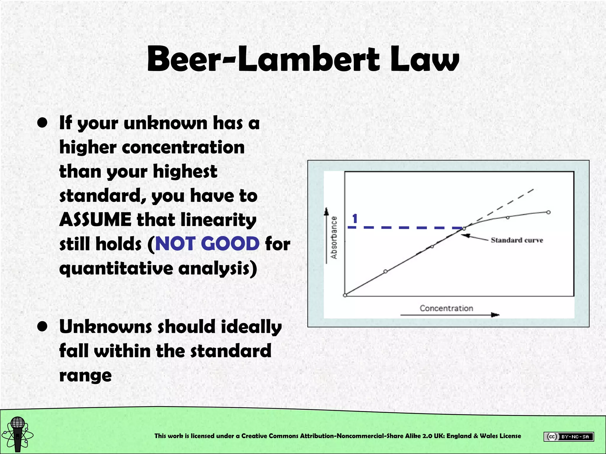
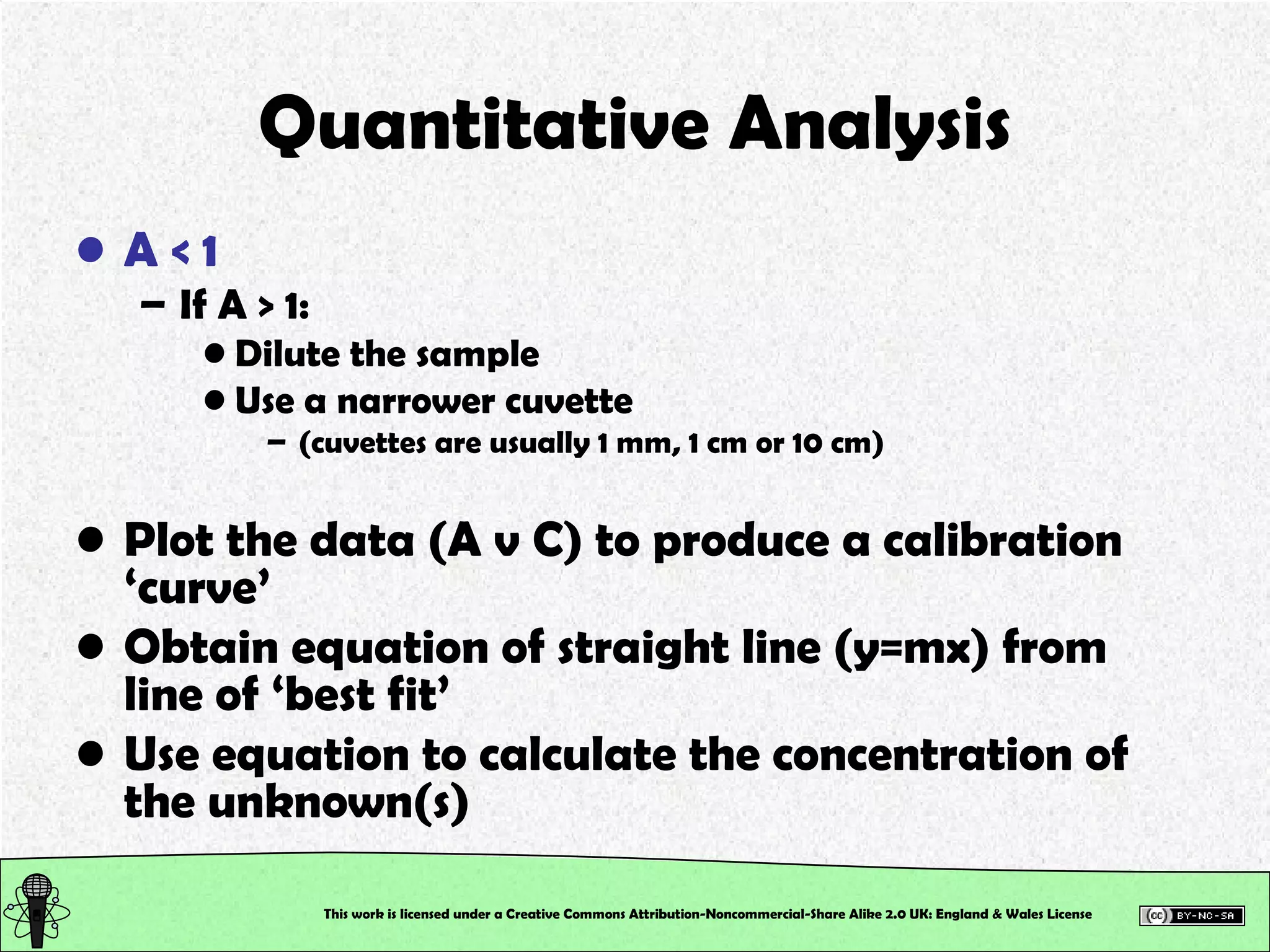
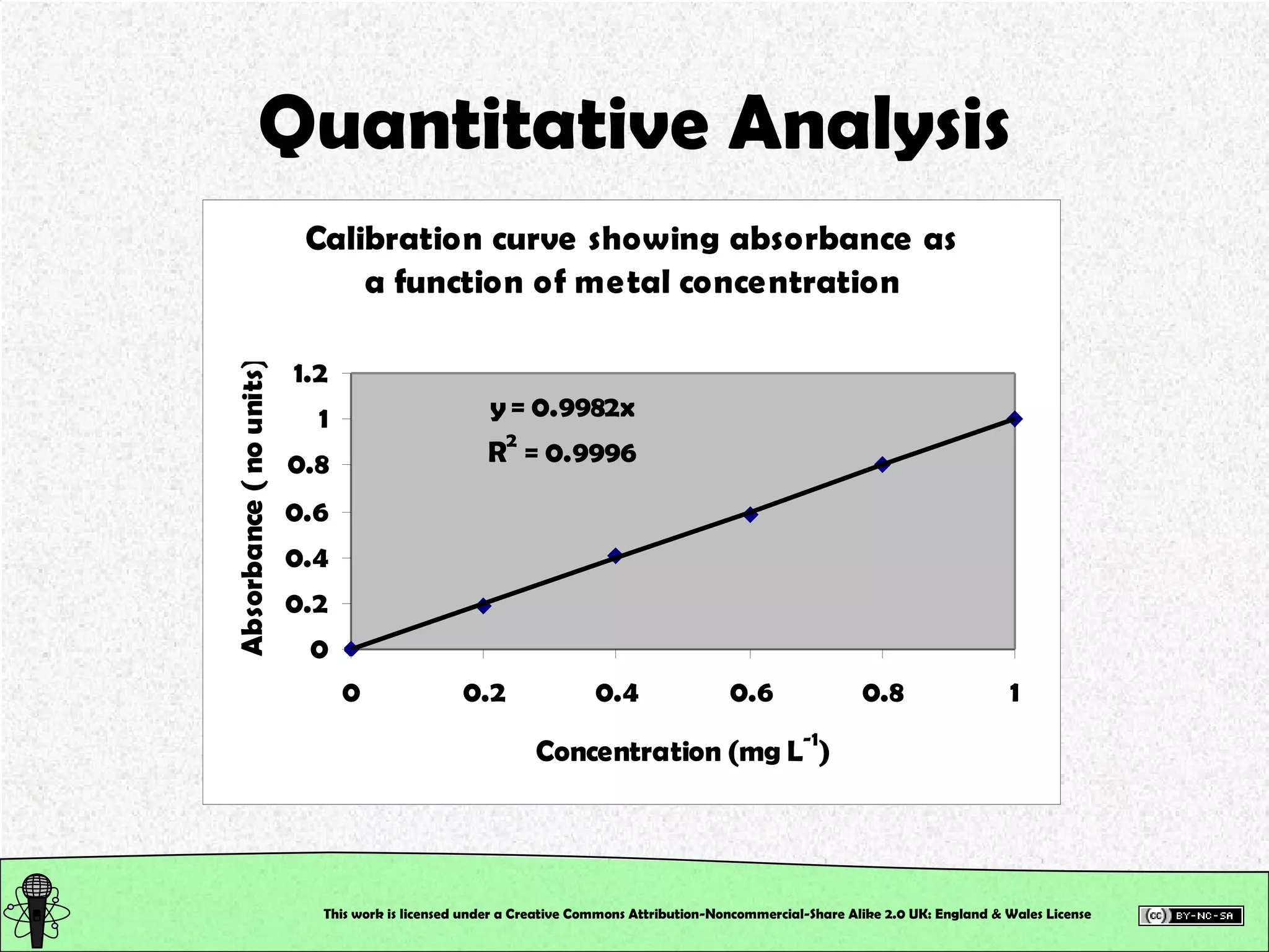
3. The Practical Determine the thiocyanate (SCN - ) in a sample of your saliva using a colourimetric method of analysis Calibration curve to determine the [SCN - ] of the unknowns This was ALL completed in the practical class Some of your absorbance values may have been higher than the absorbance values of your top standards… is this a problem???? This work is licensed under a Creative Commons Attribution-Noncommercial-Share Alike 2.0 UK: England & Wales License

4. This work is licensed under a Creative Commons Attribution-Noncommercial-Share Alike 2.0 UK: England & Wales License Types of data QUALITATIVE Non numerical i.e what is present? QUANTITATIVE Numerical: i.e. How much is present?

5. Beer-Lambert Law Beers Law states that absorbance is proportional to concentration over a certain concentration range A =  cl A = absorbance  = molar extinction coefficient (M -1 cm -1 or mol -1 L cm -1 ) c = concentration (M or mol L -1 ) l = path length (cm) (width of cuvette) This work is licensed under a Creative Commons Attribution-Noncommercial-Share Alike 2.0 UK: England & Wales License

6. Beer-Lambert Law Beer’s law is valid at low concentrations, but breaks down at higher concentrations For linearity, A < 1 This work is licensed under a Creative Commons Attribution-Noncommercial-Share Alike 2.0 UK: England & Wales License 1

7. Beer-Lambert Law If your unknown has a higher concentration than your highest standard, you have to ASSUME that linearity still holds ( NOT GOOD for quantitative analysis) Unknowns should ideally fall within the standard range This work is licensed under a Creative Commons Attribution-Noncommercial-Share Alike 2.0 UK: England & Wales License 1

8. Quantitative Analysis A < 1 If A > 1: Dilute the sample Use a narrower cuvette (cuvettes are usually 1 mm, 1 cm or 10 cm) Plot the data (A v C) to produce a calibration ‘curve’ Obtain equation of straight line (y=mx) from line of ‘best fit’ Use equation to calculate the concentration of the unknown(s) This work is licensed under a Creative Commons Attribution-Noncommercial-Share Alike 2.0 UK: England & Wales License

9. Quantitative Analysis This work is licensed under a Creative Commons Attribution-Noncommercial-Share Alike 2.0 UK: England & Wales License

10. Statistical Analysis This work is licensed under a Creative Commons Attribution-Noncommercial-Share Alike 2.0 UK: England & Wales License

11. This work is licensed under a Creative Commons Attribution-Noncommercial-Share Alike 2.0 UK: England & Wales License Mean The mean provides us with a typical value which is representative of a distribution

12. Normal Distribution This work is licensed under a Creative Commons Attribution-Noncommercial-Share Alike 2.0 UK: England & Wales License

13. Mean and Standard Deviation This work is licensed under a Creative Commons Attribution-Noncommercial-Share Alike 2.0 UK: England & Wales License MEAN

14. Standard Deviation Measures the variation of the samples: Population std (  ) Sample std (s)  = √(  (x i – µ ) 2 /n) s =√(  (x i – µ ) 2 /(n-1)) This work is licensed under a Creative Commons Attribution-Noncommercial-Share Alike 2.0 UK: England & Wales License

15.  or s? In forensic analysis, the rule of thumb is: If n > 15 use  If n < 15 use s This work is licensed under a Creative Commons Attribution-Noncommercial-Share Alike 2.0 UK: England & Wales License

16. Absolute Error and Error % Absolute Error Experimental value – True Value Error % This work is licensed under a Creative Commons Attribution-Noncommercial-Share Alike 2.0 UK: England & Wales License

17. Confidence limits This work is licensed under a Creative Commons Attribution-Noncommercial-Share Alike 2.0 UK: England & Wales License 1  = 68% 2  = 95% 2.5  = 98% 3  = 99.7%

18. Control Data Work out the mean and standard deviation of the control data Use only 1 value per group Which std is it?  or s? This will tell us how precise your work is in the lab This work is licensed under a Creative Commons Attribution-Noncommercial-Share Alike 2.0 UK: England & Wales License

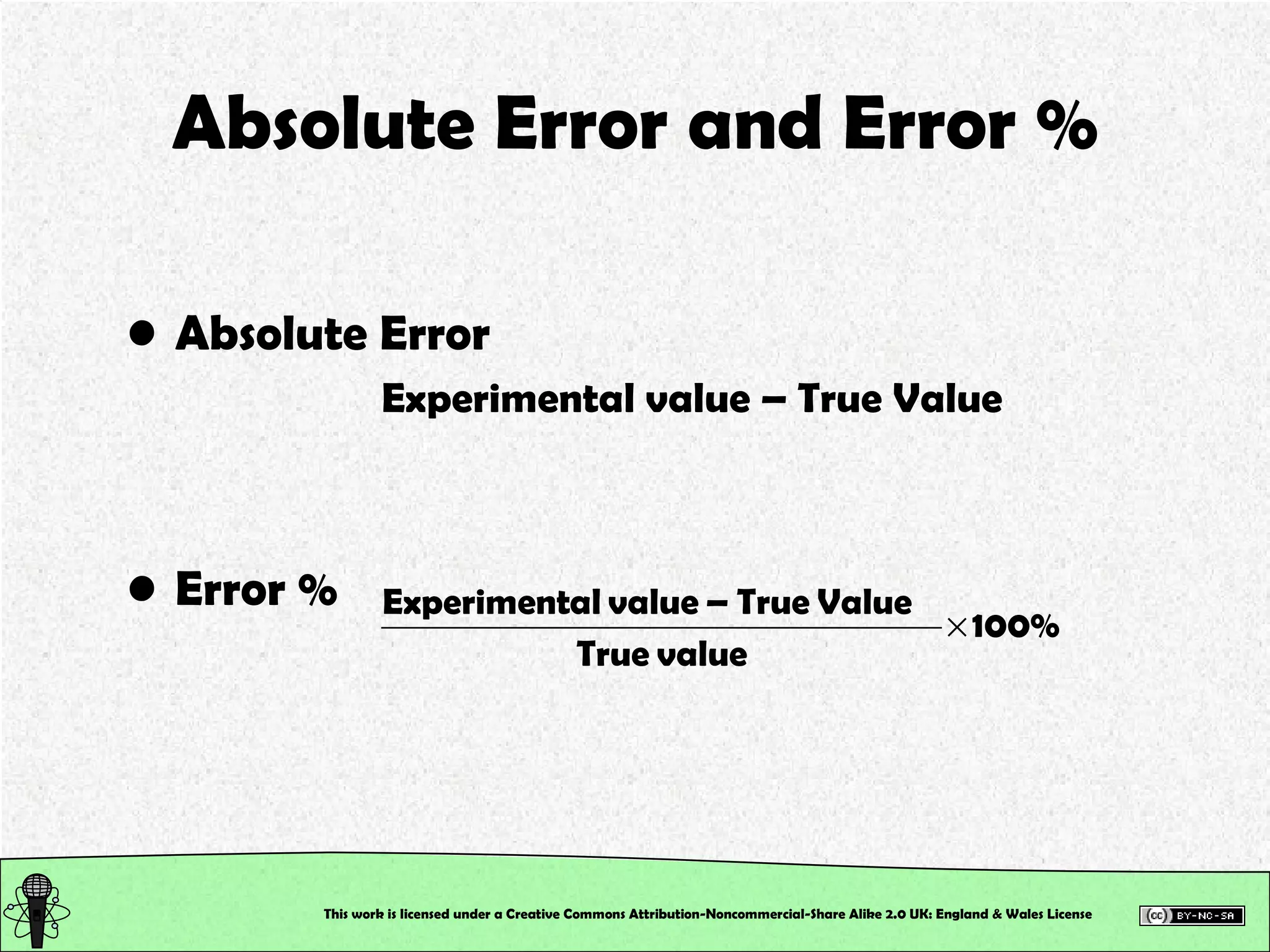
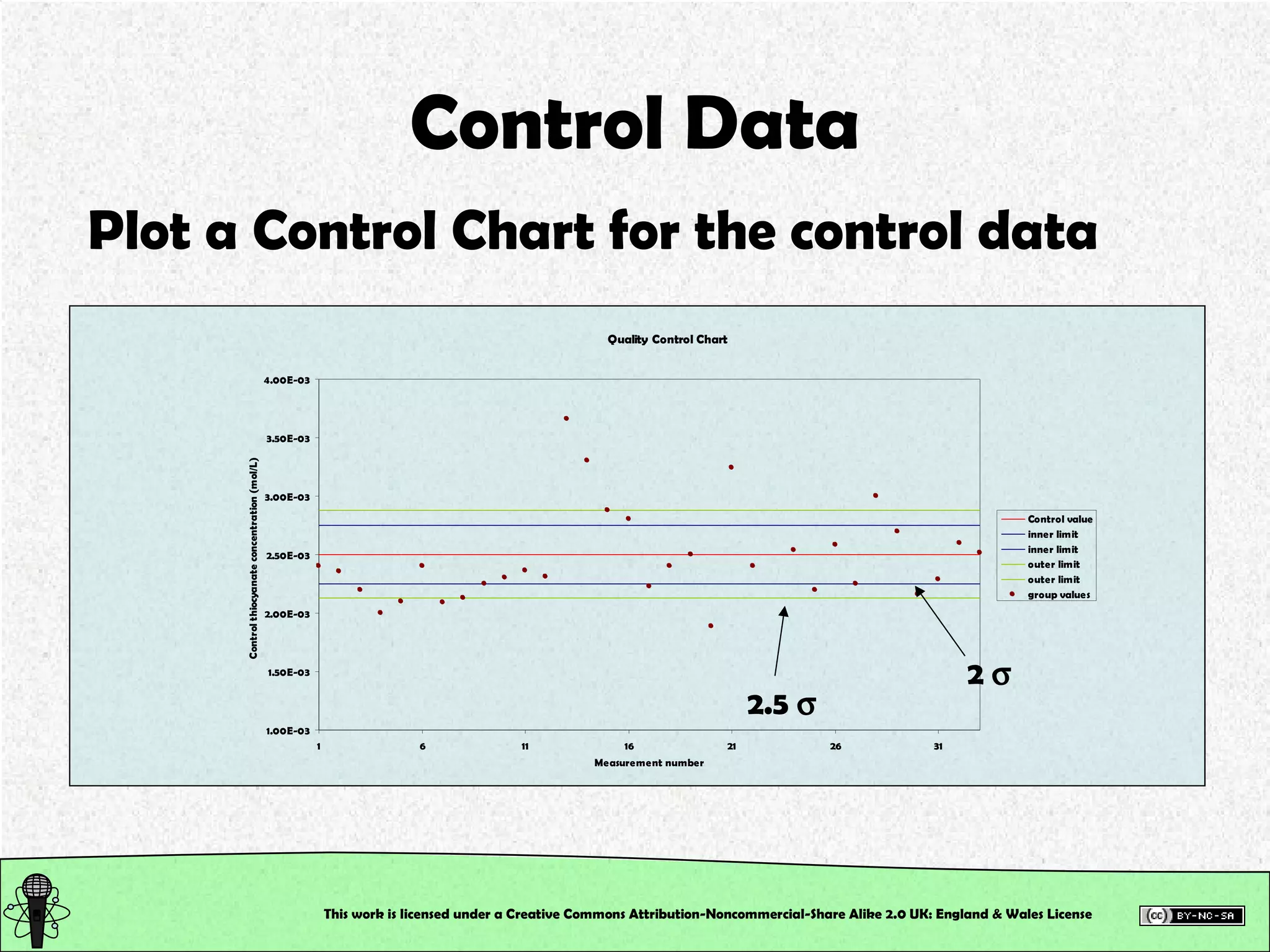
19. Control Data Calculate the Absolute Error and the Error % True value of [SCN – ] in the control = 2.0 x 10 –3 M This will tell us how accurately you work, and hence how good your calibration is!!! This work is licensed under a Creative Commons Attribution-Noncommercial-Share Alike 2.0 UK: England & Wales License

20. Control Data Plot a Control Chart for the control data This work is licensed under a Creative Commons Attribution-Noncommercial-Share Alike 2.0 UK: England & Wales License 2.5  2 

21. Significance Divide the data into six groups: Smokers Non-smokers Male Female Meat-eaters Rabbits Work out the mean and std for each group (  or s?) This work is licensed under a Creative Commons Attribution-Noncommercial-Share Alike 2.0 UK: England & Wales License

22. Significance Plot the values on a bar chart Add error bars (y-axis) at the 95% confidence limit – 2.0  This work is licensed under a Creative Commons Attribution-Noncommercial-Share Alike 2.0 UK: England & Wales License

23. Significance This work is licensed under a Creative Commons Attribution-Noncommercial-Share Alike 2.0 UK: England & Wales License

24. Identifying Significance In the most simplistic terms: If there is no overlap of error bars between two groups, you can be fairly sure the difference in means is significant This work is licensed under a Creative Commons Attribution-Noncommercial-Share Alike 2.0 UK: England & Wales License

25. This work is licensed under a Creative Commons Attribution-Noncommercial-Share Alike 2.0 UK: England & Wales License Acknowledgements JISC HEA Centre for Educational Research and Development School of natural and applied sciences School of Journalism SirenFM http://tango.freedesktop.org