Download as PDF, PPTX

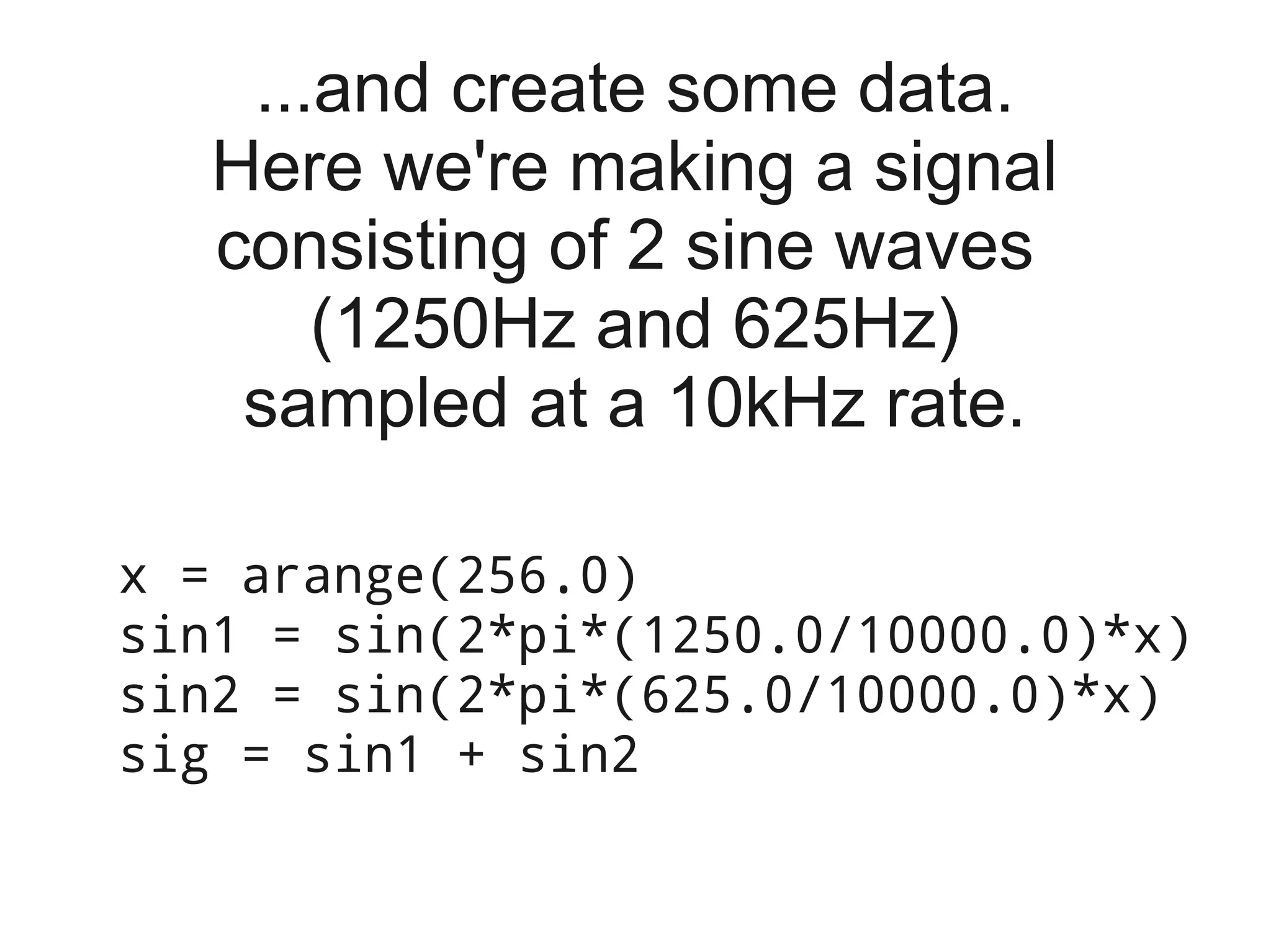
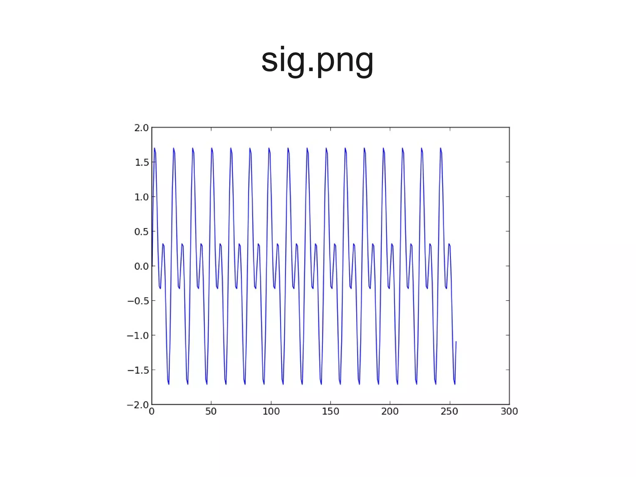
![Let's define a function to get the
data from the .wav file, and use it.
def getwavdata(file):
return scipy.io.wavfile.read(file)[1]
audio = getwavdata('flute.wav')
# more detail on scipy.io.wavfile.read
# in sigproc-outline.py, lines 117-123](https://image.slidesharecdn.com/sigproc-selfstudy-130318120948-phpapp01/75/Digital-signal-processing-through-speech-hearing-and-Python-31-2048.jpg)
![Now let's see what this looks like in
the time domain. We've got a lot of
data points, so we'll only plot the
beginning of the signal here.
makegraph(audio[0:1024], 'flute.png')](https://image.slidesharecdn.com/sigproc-selfstudy-130318120948-phpapp01/75/Digital-signal-processing-through-speech-hearing-and-Python-33-2048.jpg)

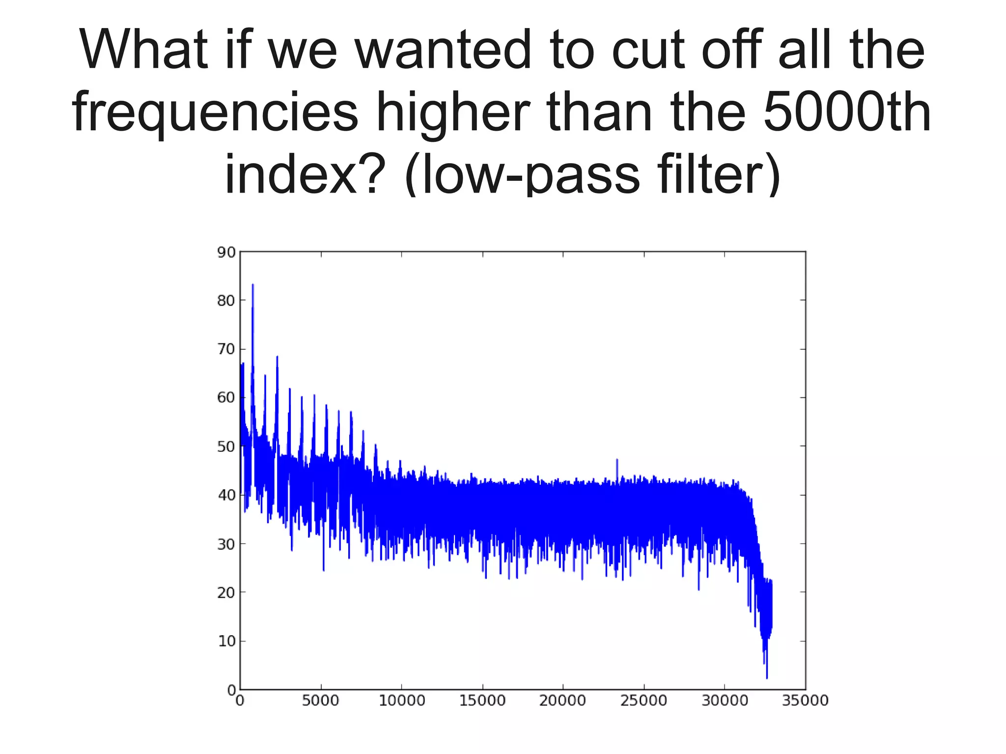
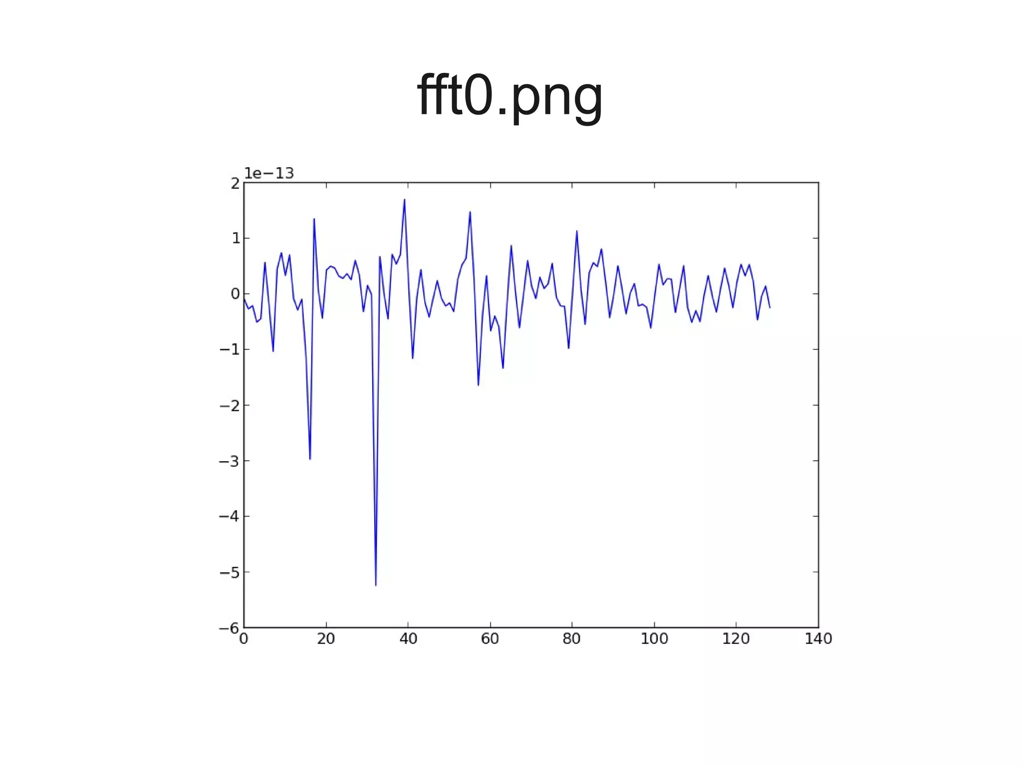
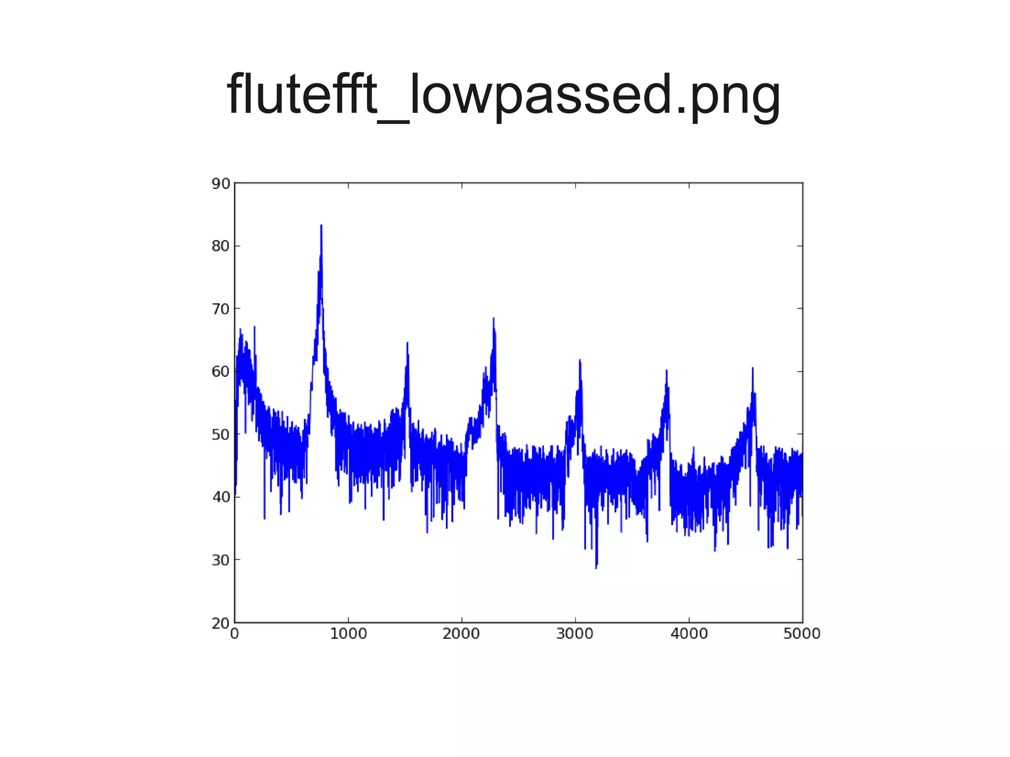
![Implement and plot the low-pass
filter in the frequency domain...
# zero out all frequencies above
# the 5000th index
# (BONUS: what frequency does this
# correspond to?)
flutefft[5000:] = 0
# plot on decibel (dB) scale
makegraph(10*log10(abs(flutefft)),
'flutefft_lowpassed.png')](https://image.slidesharecdn.com/sigproc-selfstudy-130318120948-phpapp01/75/Digital-signal-processing-through-speech-hearing-and-Python-63-2048.jpg)

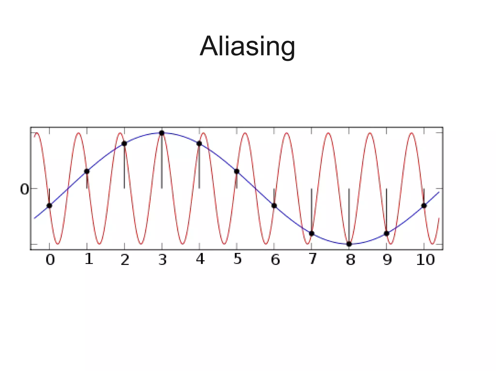
This document is a tutorial on digital signal processing using Python, focusing on audio analysis and manipulation. It covers concepts like Fourier transforms, signal visualization, sampling, and filtering, while providing hands-on coding exercises that encourage interactive learning. The tutorial is designed for participants with basic knowledge of Python and aims to accomplish in three hours what typically takes 144 hours in a standard class.


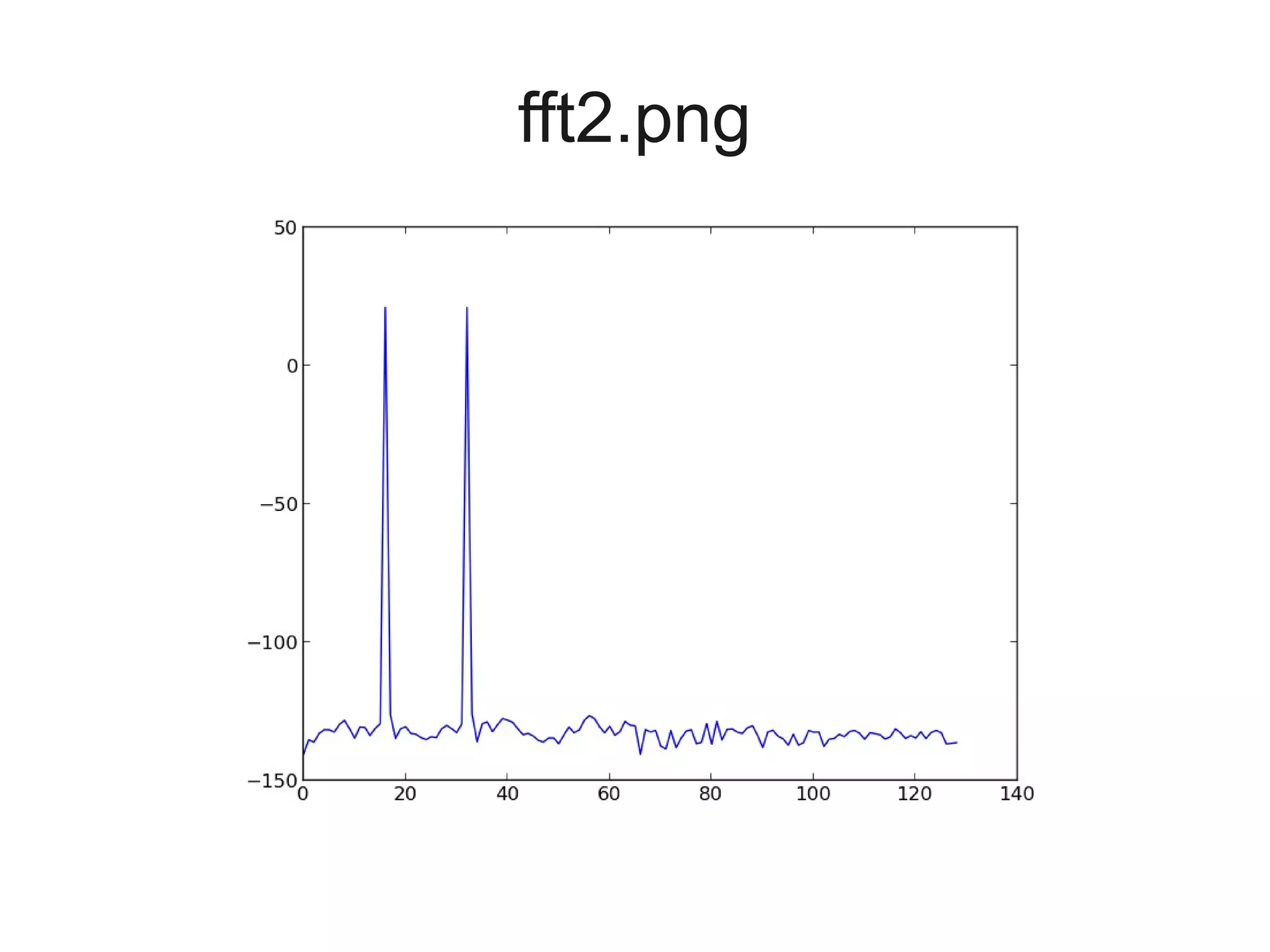
![9152018 clsdspcec411lab2 [Class Wiki at erau.us]http.docx](https://cdn.slidesharecdn.com/ss_thumbnails/9152018clsdspcec411lab2classwikiaterau-221224085308-7b1a11de-thumbnail.jpg?width=640&height=640&fit=bounds)


