Downloaded 159 times

![Linearization By Equation Inversion
Consider a transducer, that converts pressure into voltage as:
V=K [p]^0.5
V is converted into a binary no. by ADC.
DV varies as [p]^0.5.
Squaring this DV
p varies as DV*DV
Thus a program would input a sample DV and multiply it by
itself.](https://image.slidesharecdn.com/prof-150901074550-lva1-app6891/75/Signal-conditioning-condition-monitoring-using-LabView-by-Prof-shakeb-ahmad-khan-14-2048.jpg)


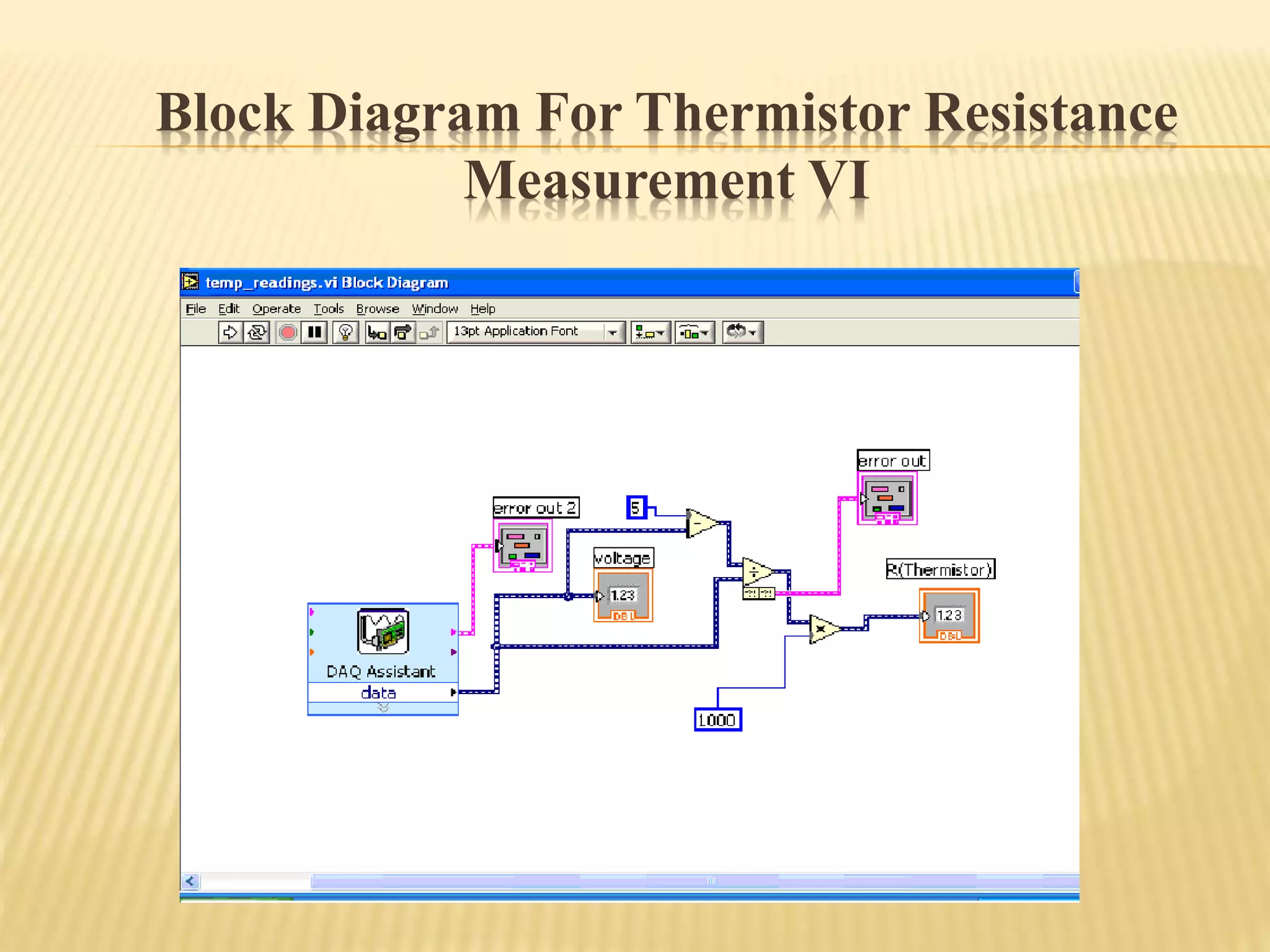
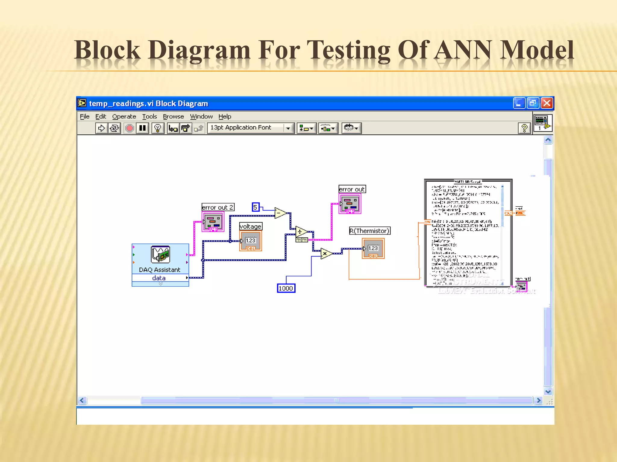

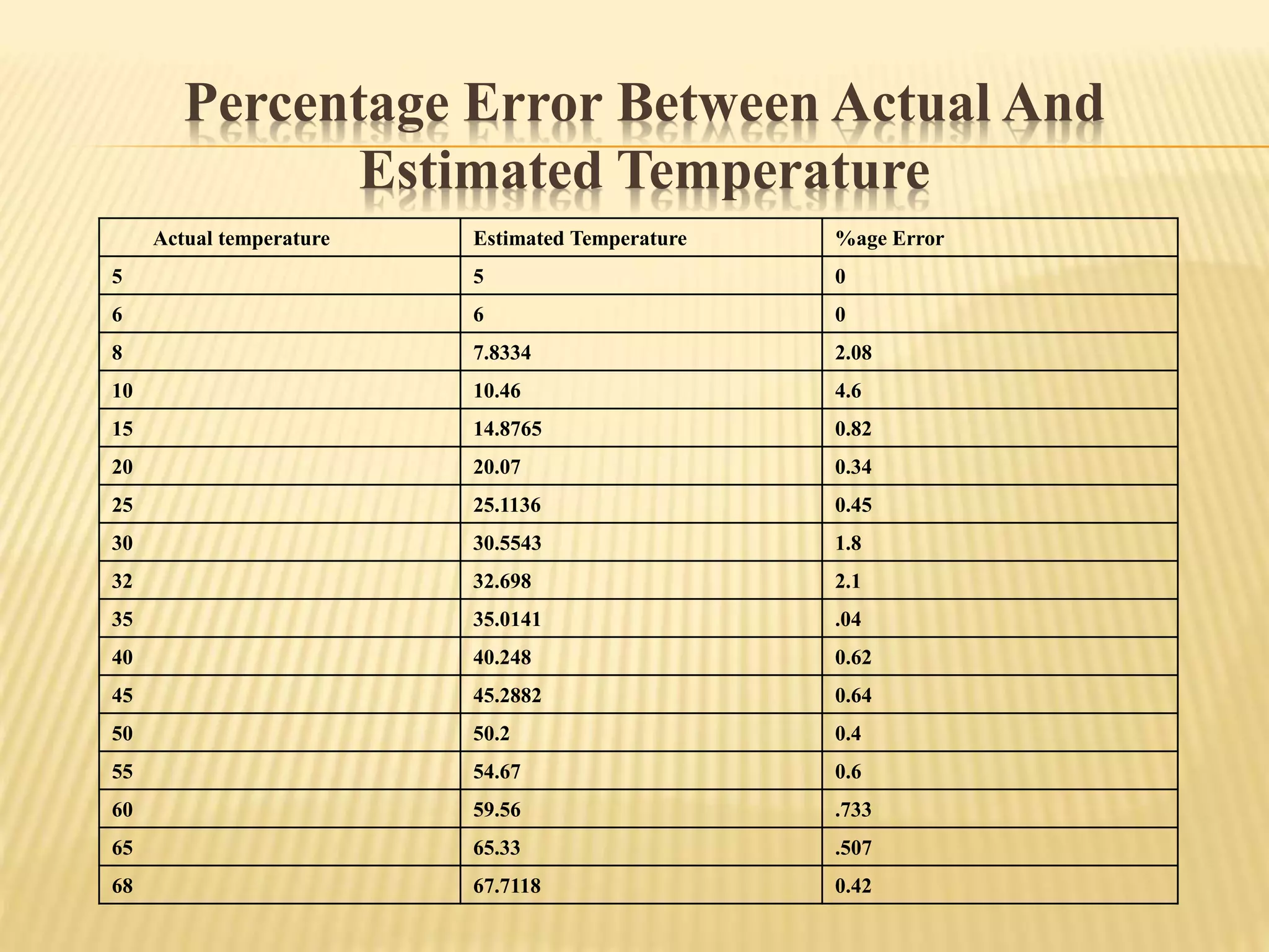

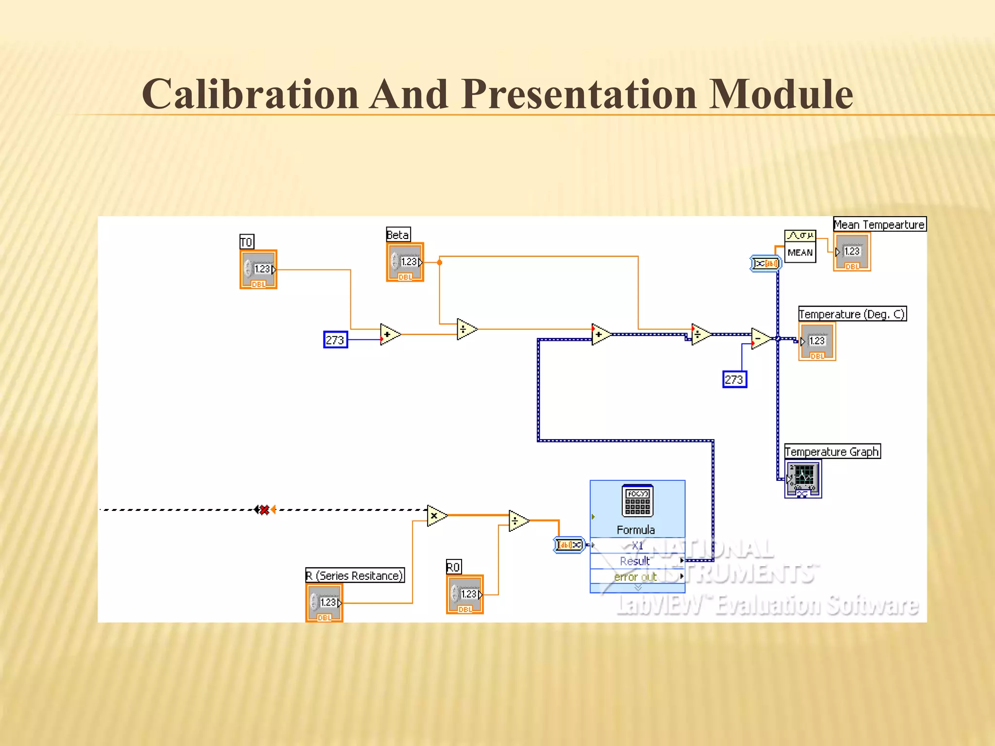
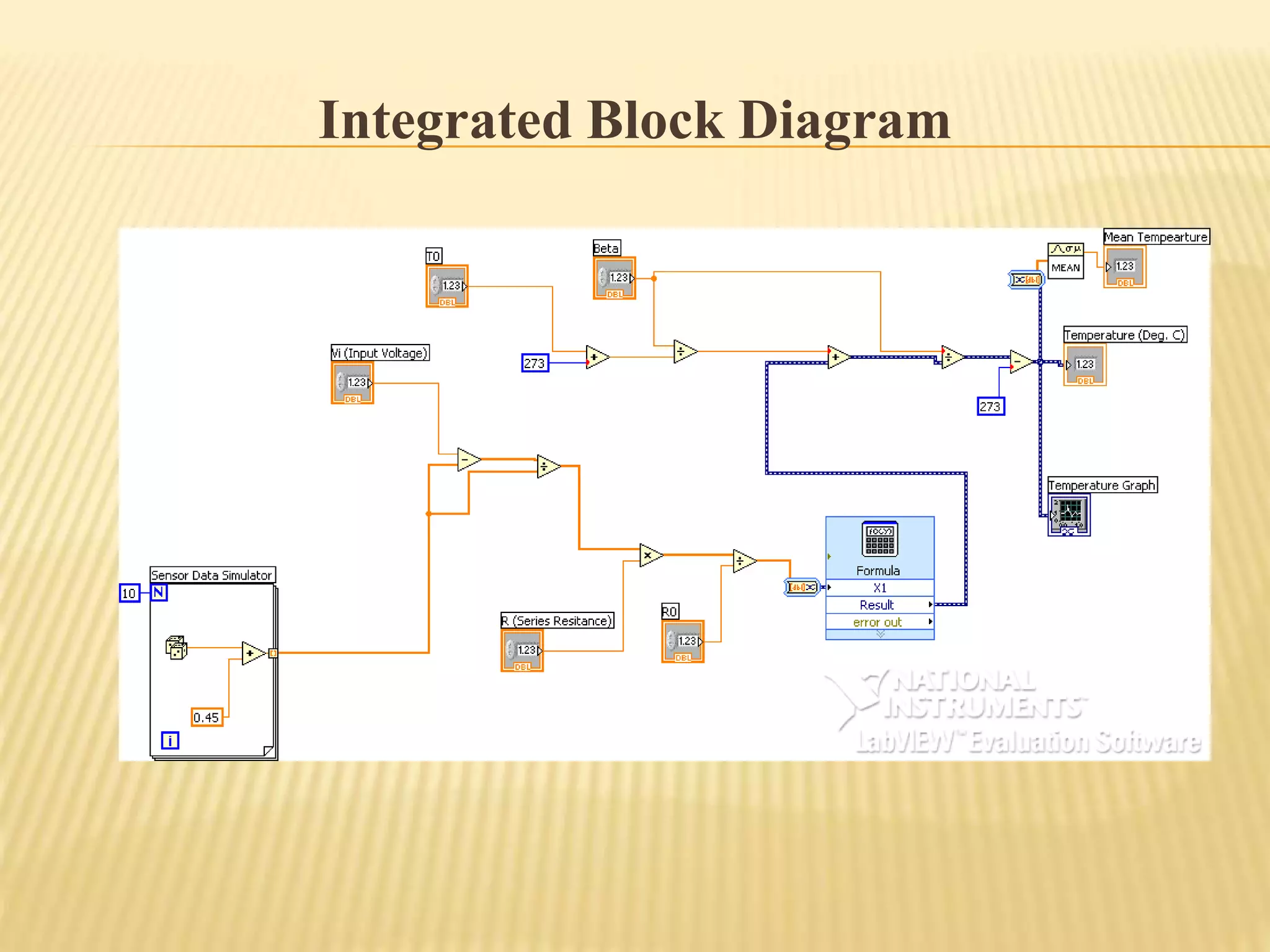
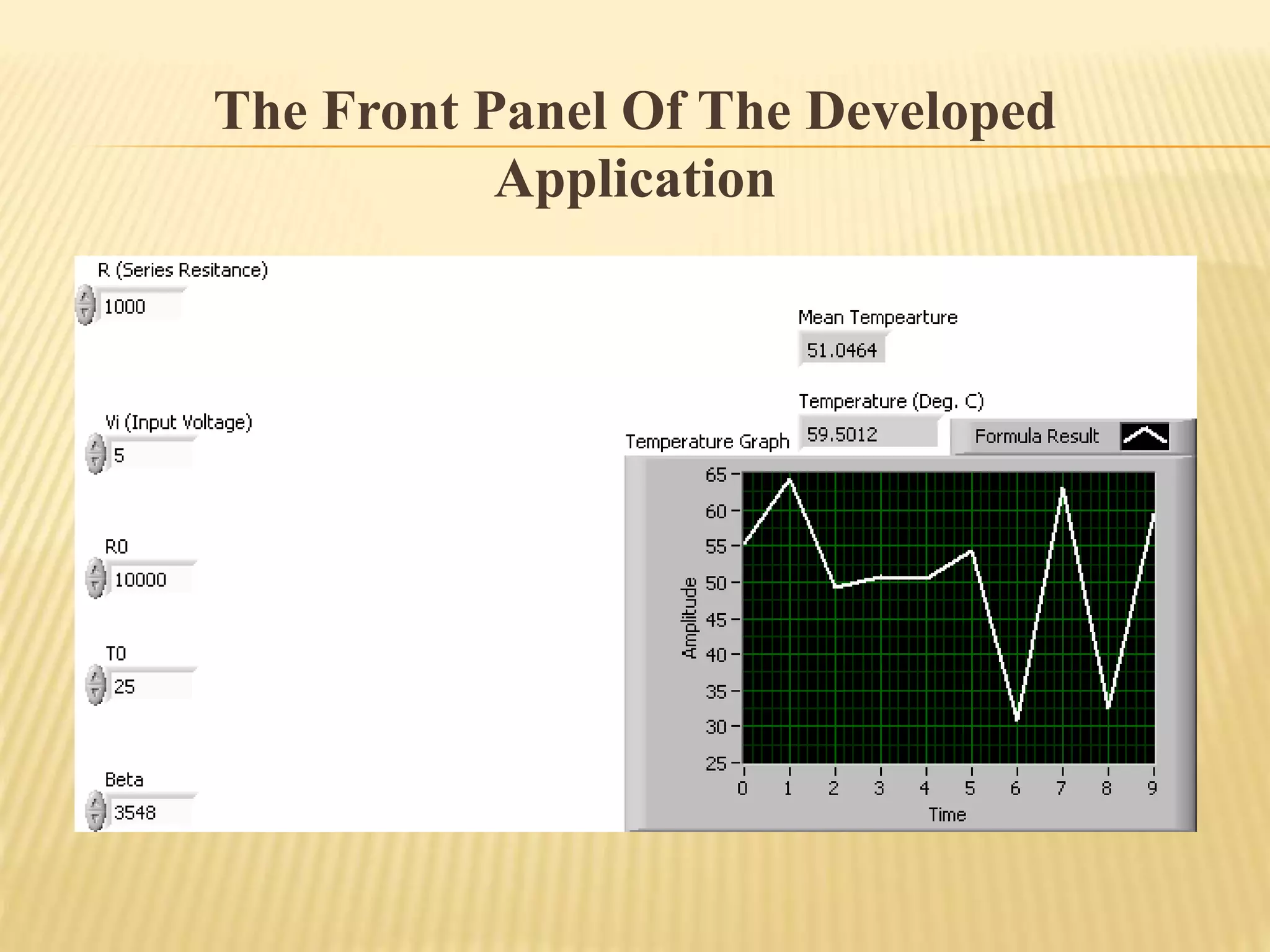
![Calibration And Presentation Module
The calibration module implements following expression:-
T = /[{ln(Rth/ R0)}+ /T0]
Where
Rth Thermistor resistance at T (K)
T Thermistor temperature (K)
R0 Resistance at T0 (K)
Thermistor characteristics constant (K)](https://image.slidesharecdn.com/prof-150901074550-lva1-app6891/75/Signal-conditioning-condition-monitoring-using-LabView-by-Prof-shakeb-ahmad-khan-41-2048.jpg)

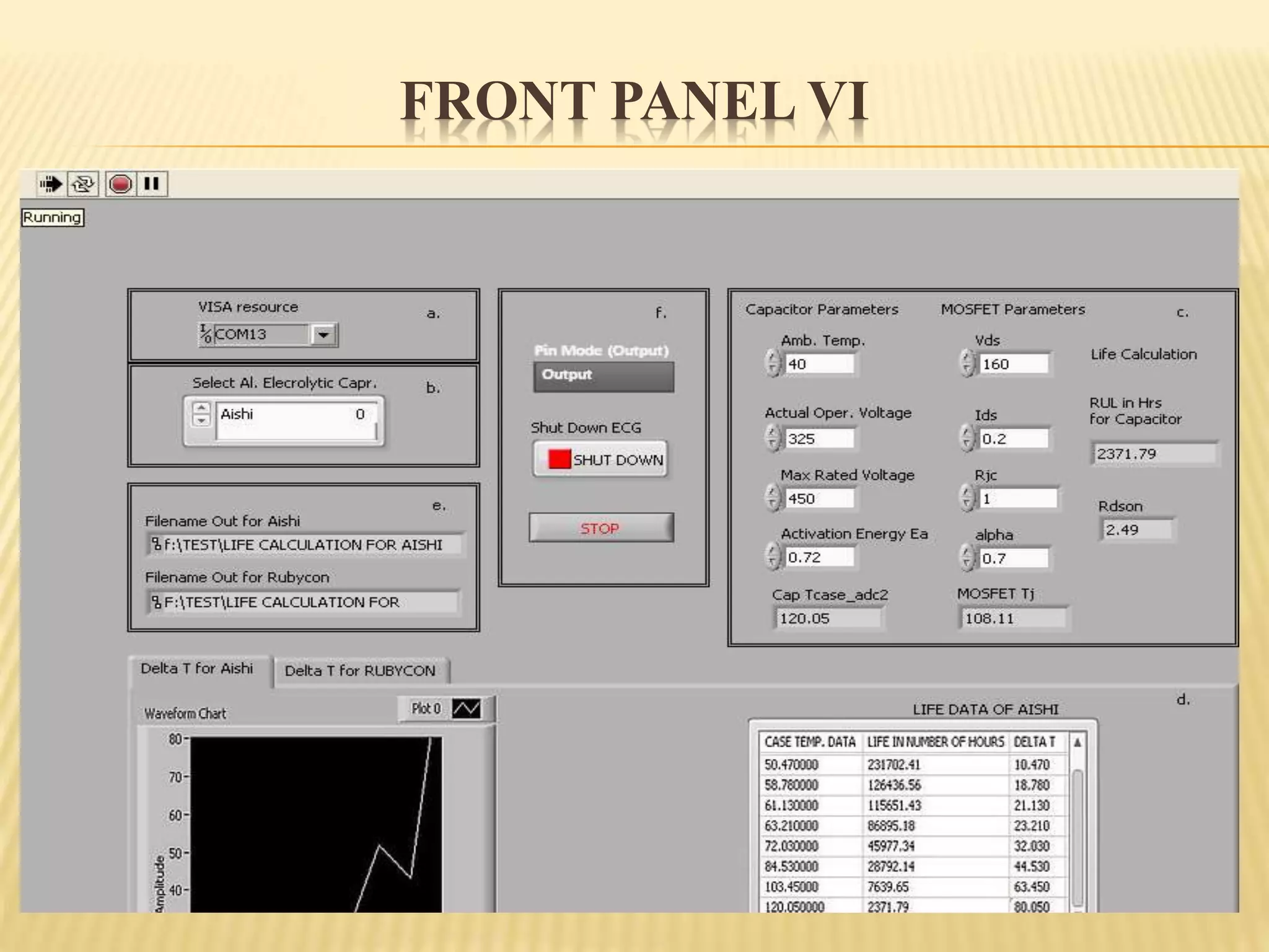
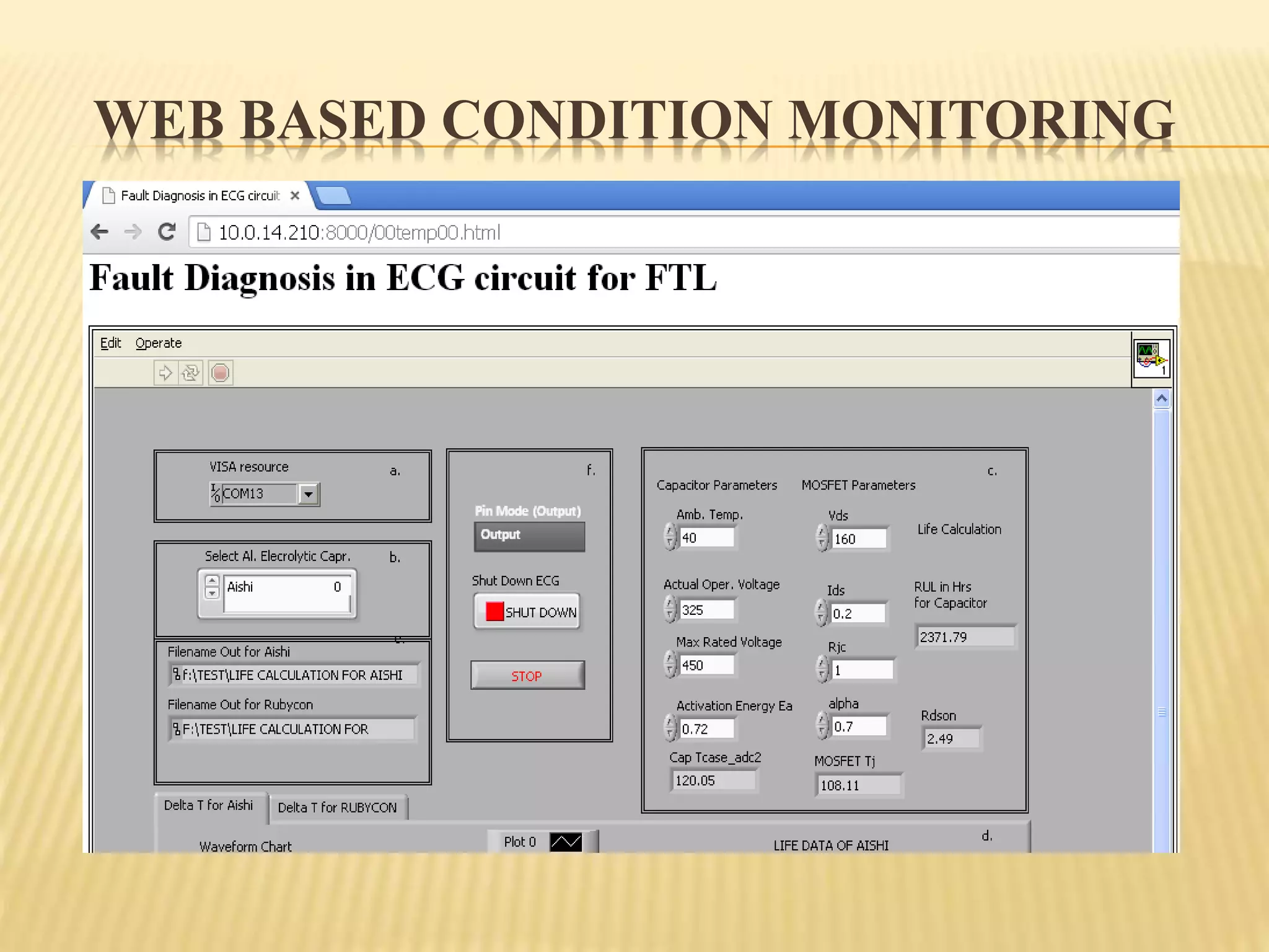
![WEB BASED CONDITION MONITORING
[MONITORING MODE]](https://image.slidesharecdn.com/prof-150901074550-lva1-app6891/75/Signal-conditioning-condition-monitoring-using-LabView-by-Prof-shakeb-ahmad-khan-57-2048.jpg)
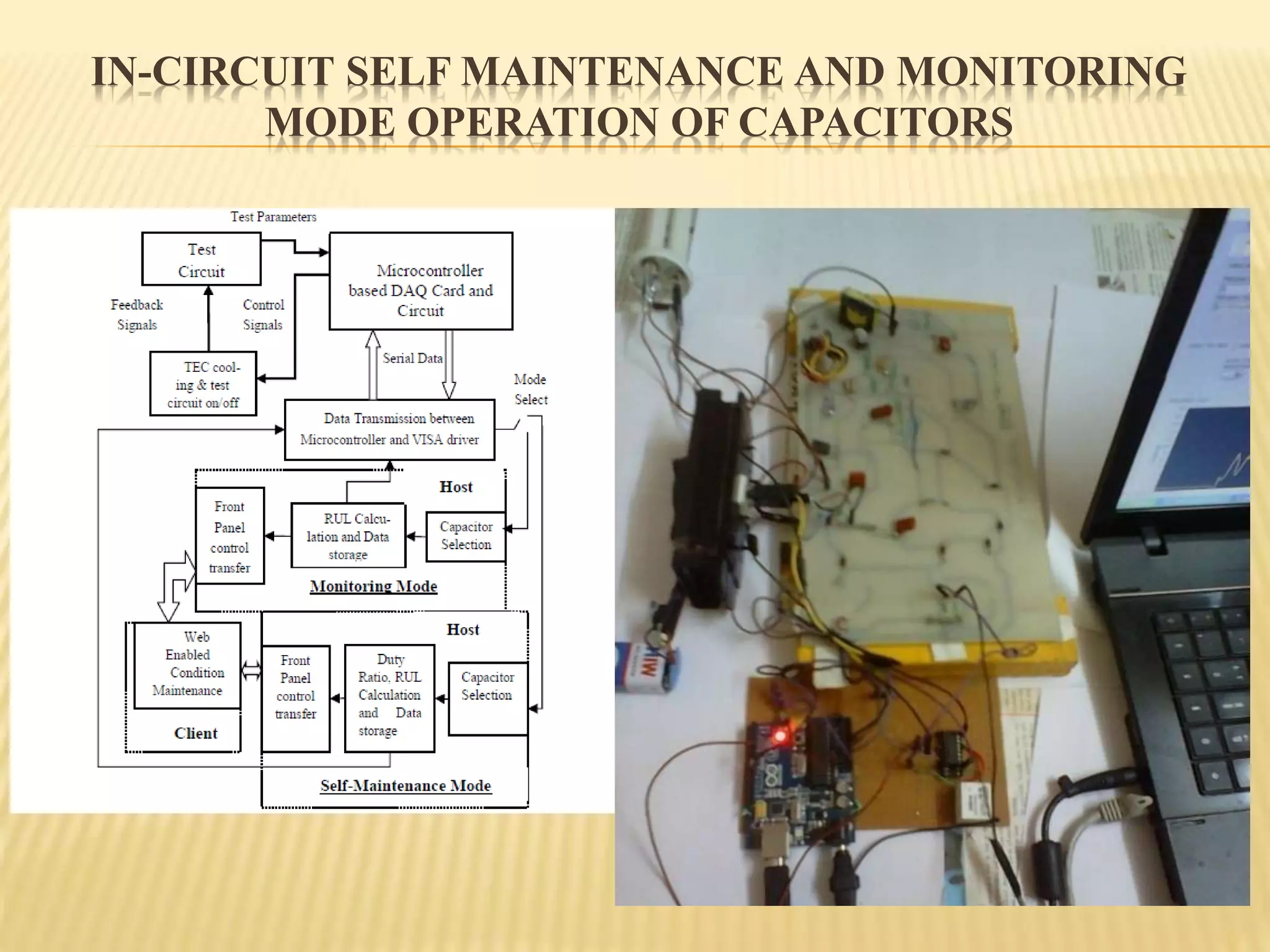
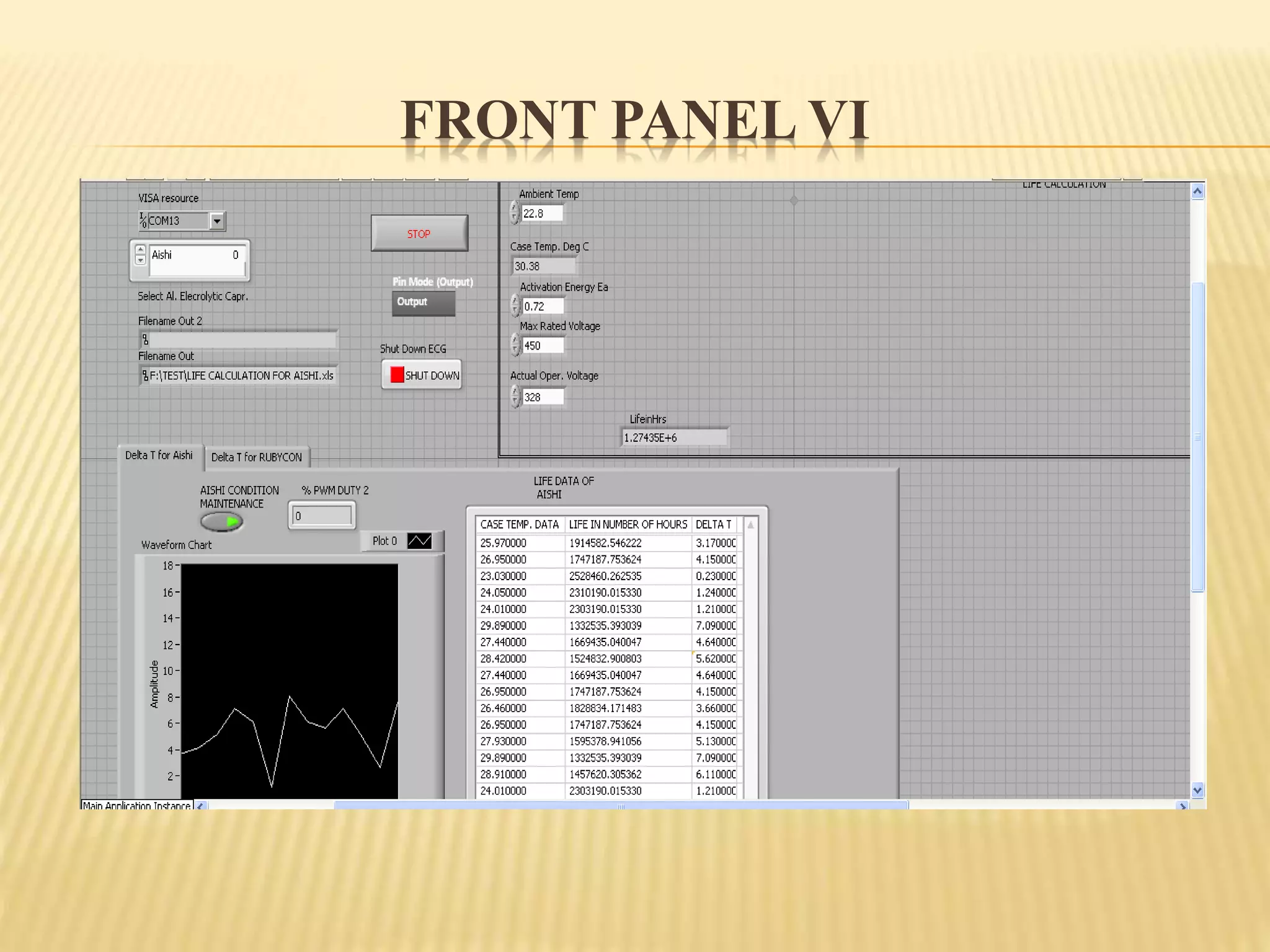
![WEB BASED CONDITION MONITORING [SELF
MAINTENANCE MODE]](https://image.slidesharecdn.com/prof-150901074550-lva1-app6891/75/Signal-conditioning-condition-monitoring-using-LabView-by-Prof-shakeb-ahmad-khan-58-2048.jpg)


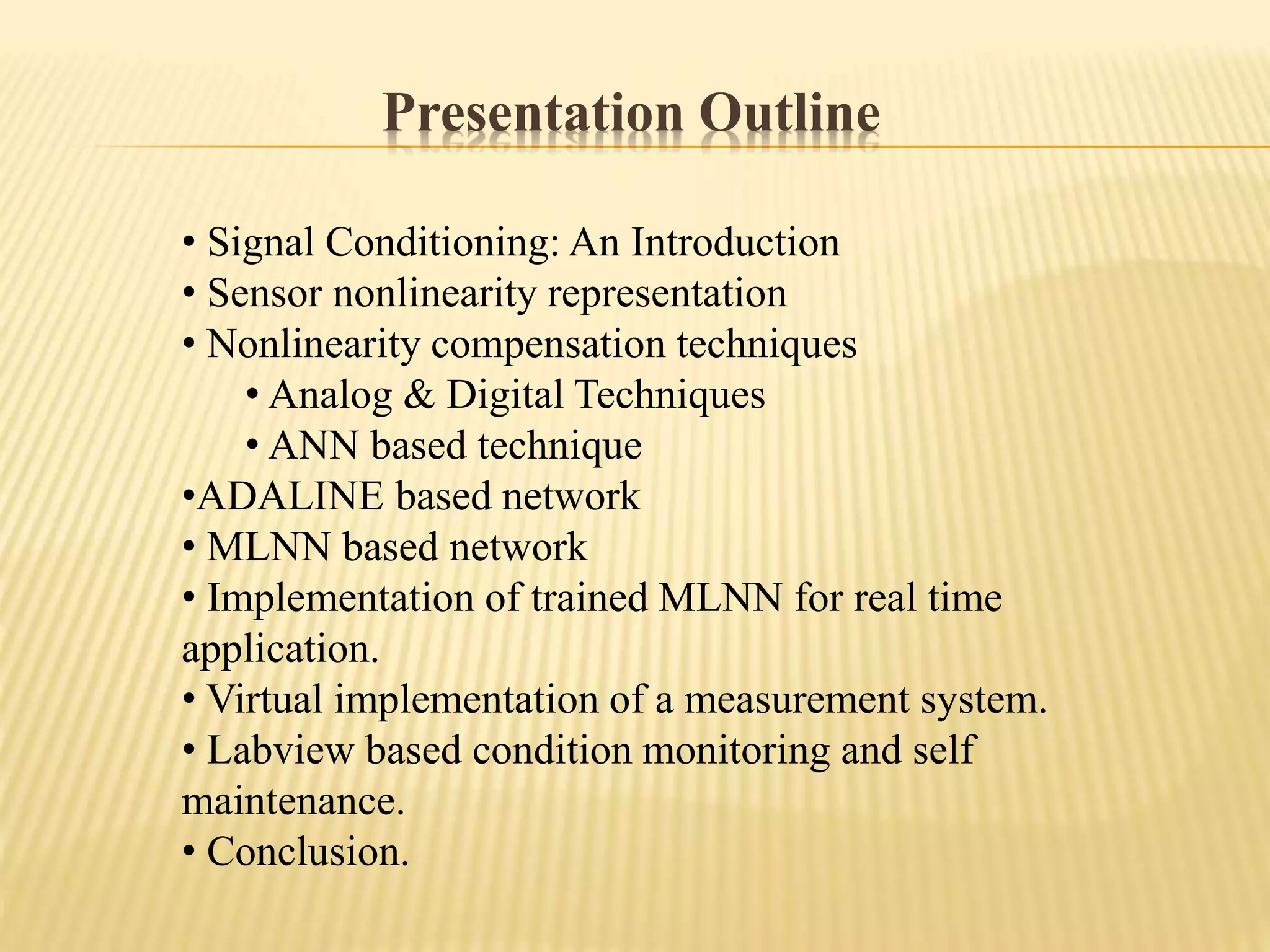
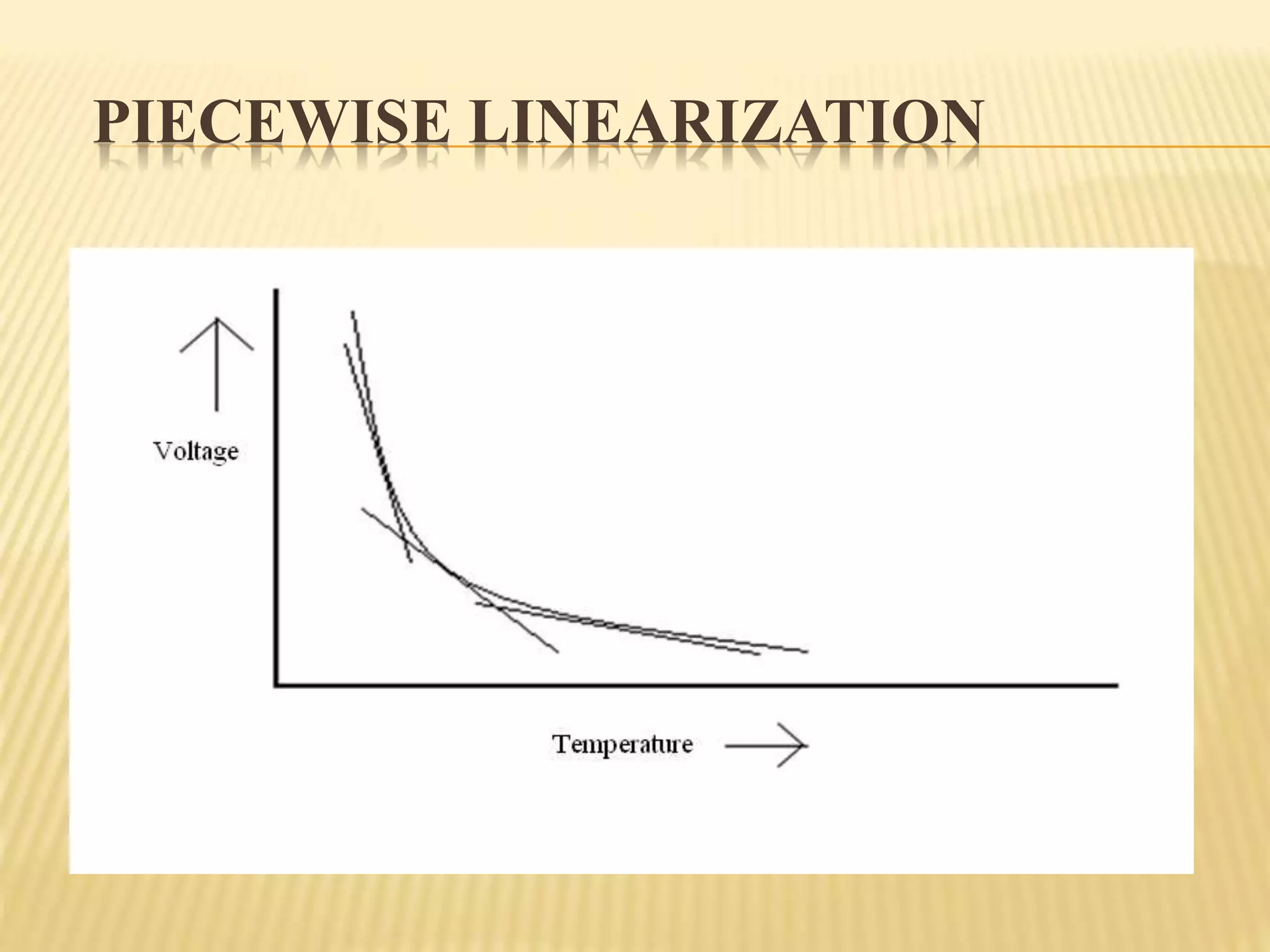
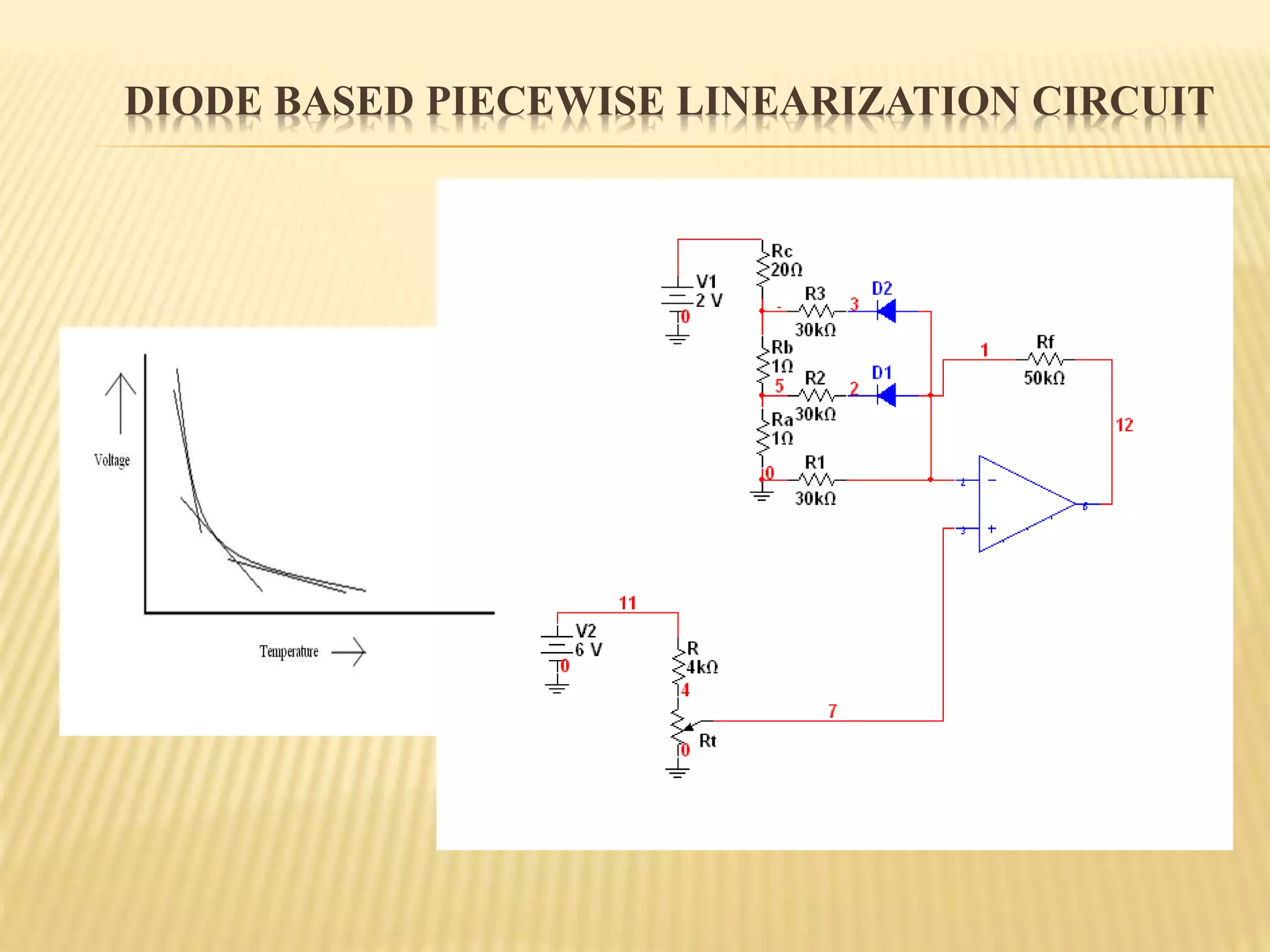
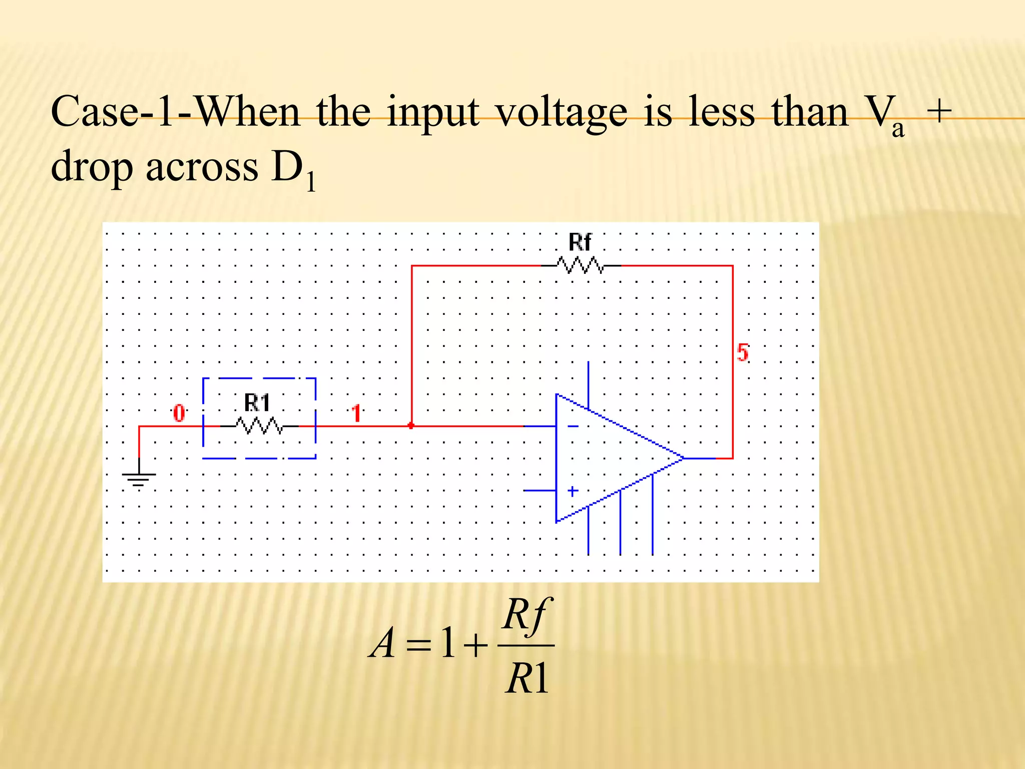
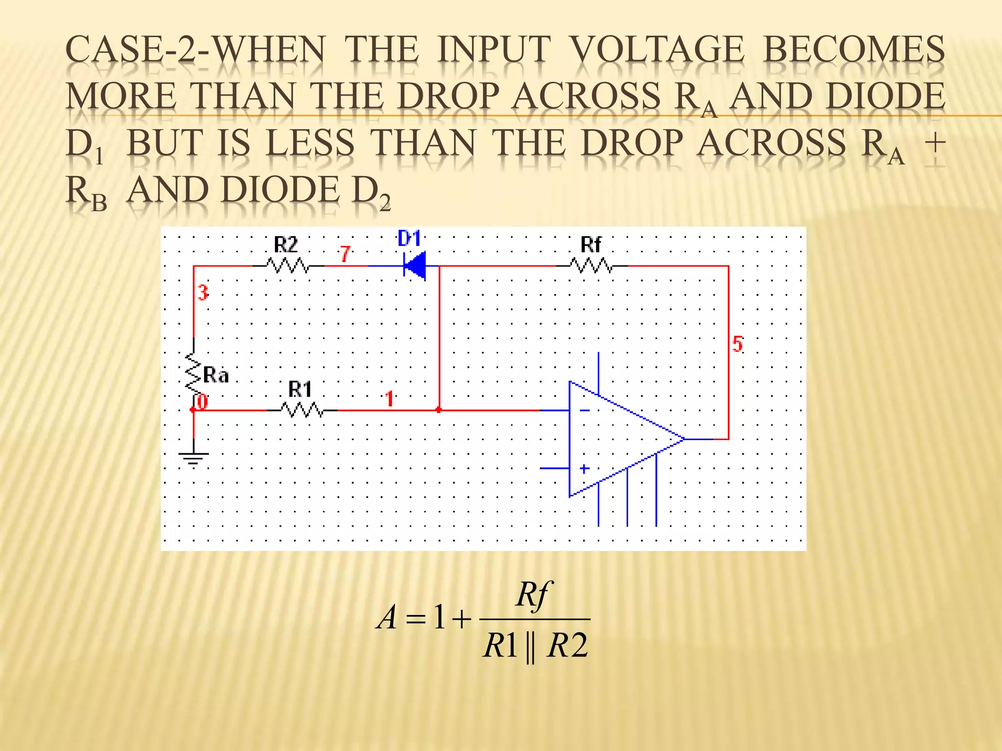
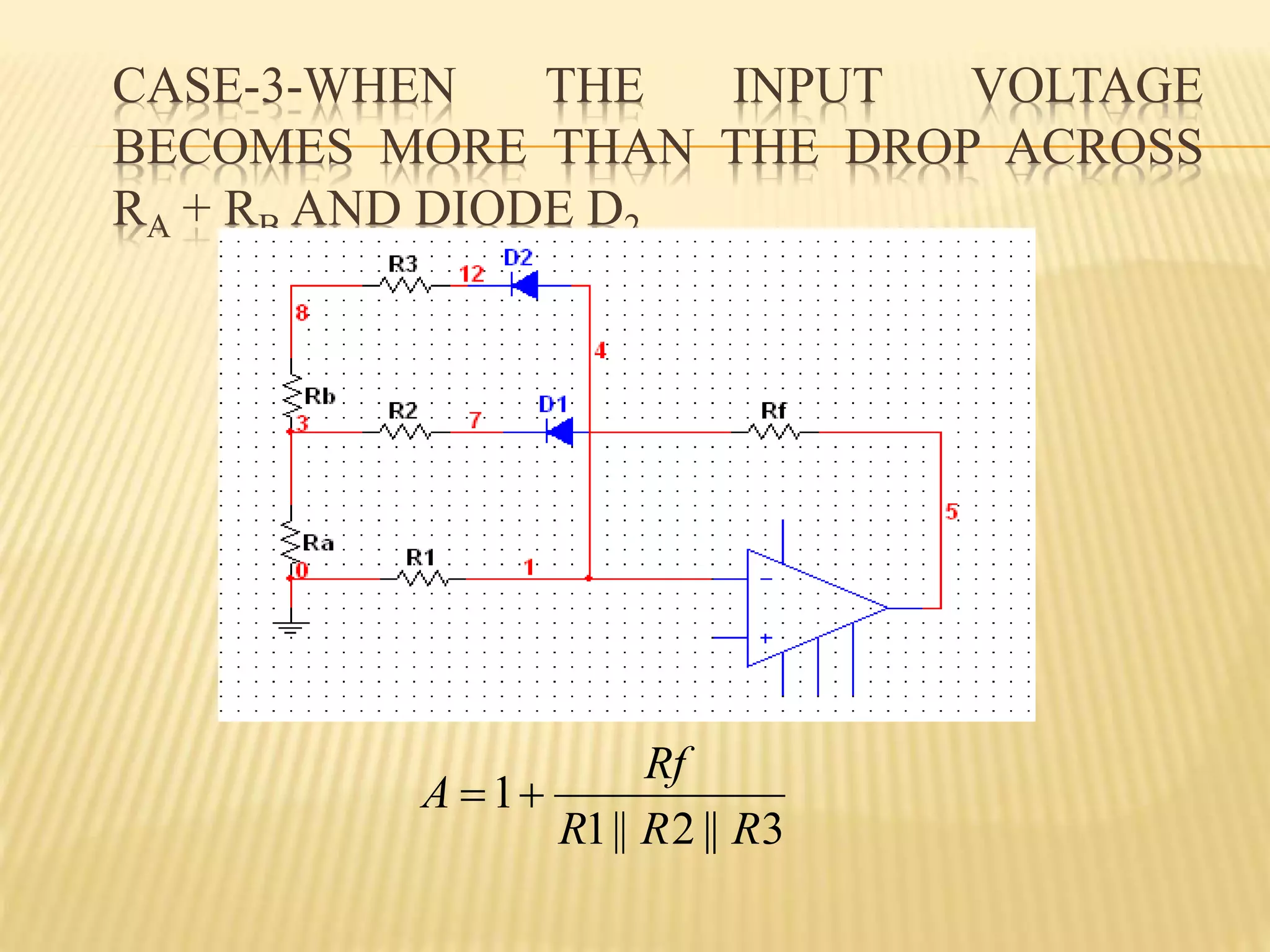
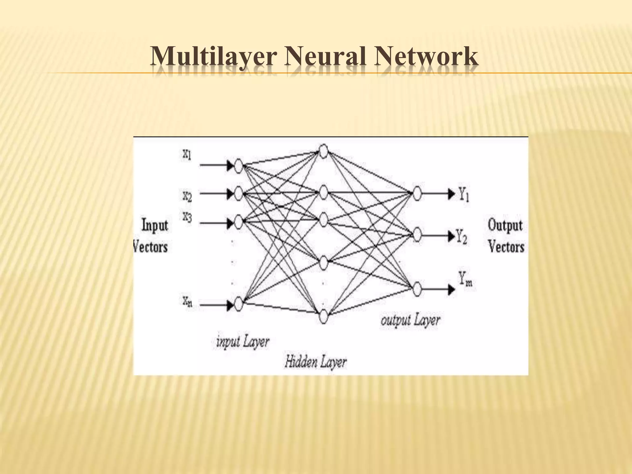
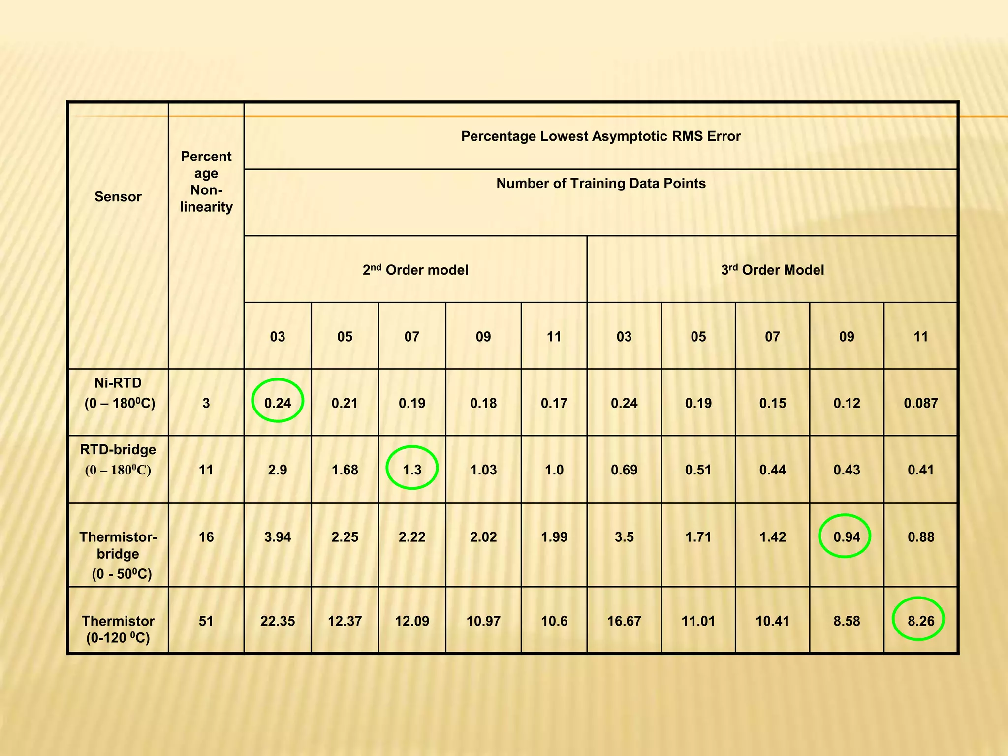
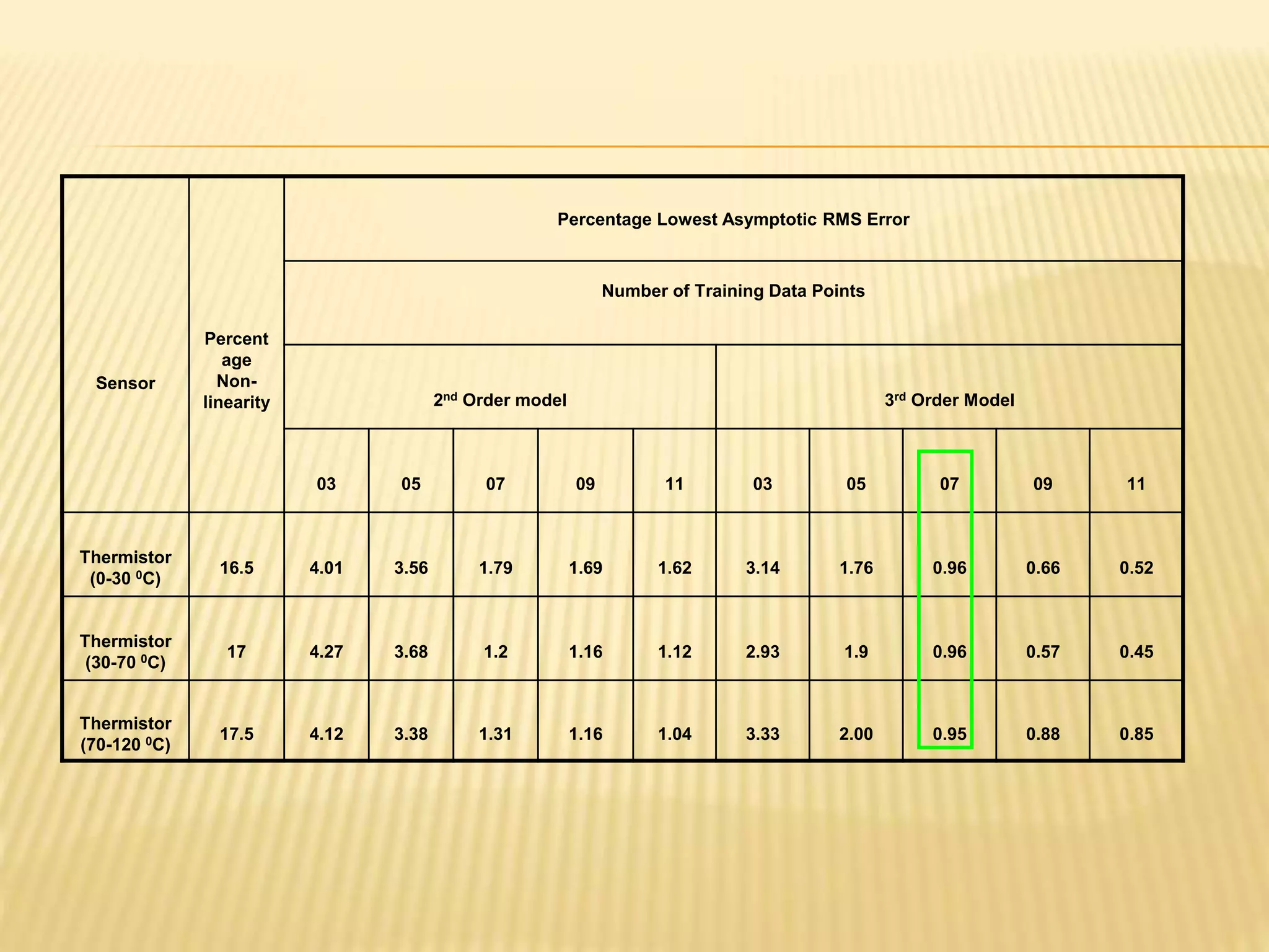
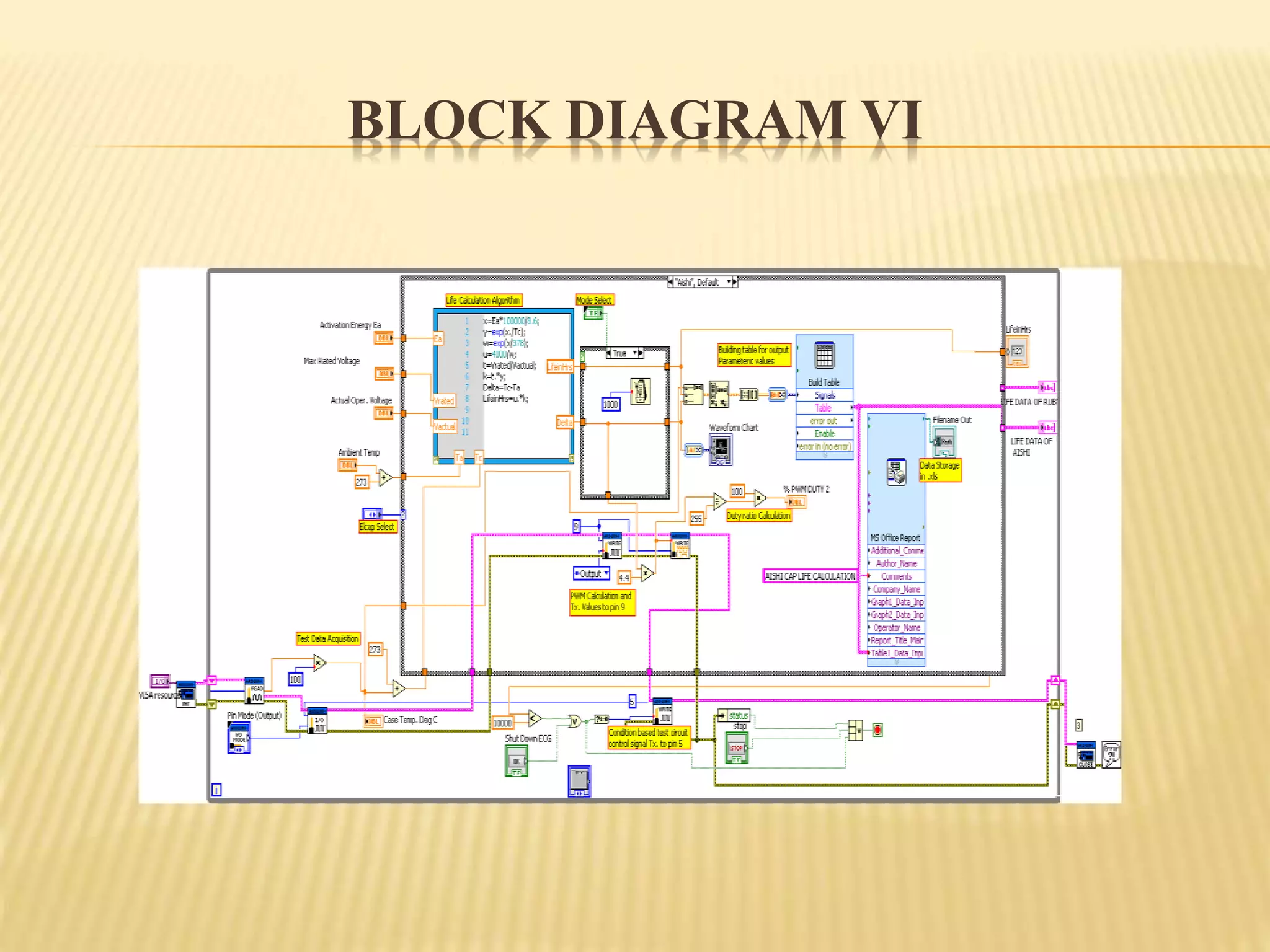
The document outlines methods for signal conditioning and nonlinearity compensation in sensor systems, detailing techniques like piecewise linearization and artificial neural networks (ANNs). It discusses the implementation of a measurement system using MATLAB and LabVIEW for real-time monitoring and self-maintenance of sensors. The conclusion emphasizes a generalized multilayer ANN method for linearization and presents a virtual temperature measurement system alongside condition monitoring practices.


![Sensor Technology Lecture 6 [Autosaved].pptx](https://cdn.slidesharecdn.com/ss_thumbnails/lecture6autosaved-250626060615-a31db175-thumbnail.jpg?width=640&height=640&fit=bounds)