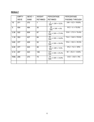
1
CODE & SUBJECT : DCC 2042 – CONCRETE AND
BRICWORK
TITLE : SIEVE TEST ( FINE AGGREGATE)
LECTURER’S NAME : PUAN HUSNA BINTI MAT SALLEH
KELAS : DKA1B
NAME REGISTRATION NO.
MUHAMAD AKMAL BIN MOHAMAD SHARIF 03DKA16F2030
AINUNYASMINE BINTI HASLAN 03DKA16F2023
NIRANDOAL A/L CHENG 03DKA16F2029
NUR AIDA BINTI ZAINOL ABIDIN 03DKA16F2027
2
OBJECTIVE
To determine a particular soil grain size distribution(GSD) THEORY : The experiment is
carried out to determine a good distribution of aggregate by using sieve and comparing
the result obtained with BS 410. The plotted distribution curve can give a clear picture of
the quality of different sizes of aggregates. A good distribution curve must be an ’Ideal
Fuller Curve’ .
APPARATUS
1. Division box size 25.4mm (1’’) and 44.45mm (13/4 )
2. 500g of dry fine aggregate.(sand)
3. Sieve size : 0.212mm.025mm,06mm,1.18mm,2.34mm.
4. Sieve pan and cover.
5. Mechanical sieve shaker
3
PROCEDURE
1. Perform a visual classification on the soil provided.
2. Inspect your sieve stack. Check for any loose screens, holes in the screens or
tears at the seams. Clean the sieve if necessary. Use a course wire brush for
larger sieve sizes, but use a soft nylon brush with smaller sieve sizes.
3. Divide the sample of fine aggregate with a division box, size 25.4mm and
course aggregate with division box size 44.45mm.
4. Weigh accurately 500g of fine aggregate.
5. Use a sieve with diameter 20.32mm to 2.4mm for fine aggregate.
6. Place your sieves in a stack of increasing sieve number- this corresponds to
decreasing opening size. The largest sieve opening should be on top, and the
pan at the bottom.
4
7. Pour the prepared aggregate sample into the top if the sieve and place the
cover tightly on top.
8. Place the sieve stacked into the sieve shaker and secure the top clamp.
When the sieve shaker has stopped, remove the sieve stack.
9. Now, record the mass of each sieve (and the pan) with it’s contents. Since
you’ve already obtained the sieve’s masses, you can now determine the
amount of soil retained on each sieve.
5
ANALYSIS
 Weight passing through :
𝑤𝑒𝑖𝑔ℎ𝑡 𝑜𝑓 𝑠𝑎𝑚𝑝𝑙𝑒 − 𝑤𝑒𝑖𝑔ℎ𝑡 𝑟𝑒𝑡𝑎𝑖𝑛𝑒𝑑
 Percentage passing through :
𝑤𝑒𝑖𝑔ℎ𝑡 𝑝𝑎𝑠𝑠𝑖𝑛𝑔 𝑡ℎ𝑟𝑜𝑢𝑔ℎ
𝑤𝑒𝑖𝑔ℎ𝑡 𝑟𝑒𝑡𝑎𝑖𝑛𝑒𝑑
× 100%
 Percentage retained :
𝑤𝑒𝑖𝑔ℎ𝑡 𝑟𝑒𝑡𝑎𝑖𝑛𝑒𝑑
𝑤𝑒𝑖𝑔ℎ𝑡 𝑜𝑓 𝑠𝑎𝑚𝑝𝑙𝑒
× 100%
6
RESULT
EMPTY
SIEVE
SIEVE +
SAND
WEIGHT
RETAINED
PERCENTAGE
RETAINED
PERCENTAGE
PASSING THROUGH
10 371 372 1 1
500
× 100 = 0.2%
100 − 0.2 = 99.8%
5 454 484 30 30
500
× 100 = 6%
99.5 − 6 = 93.8%
2.36 522 609 87 87
500
× 100 = 17.4%
93.8 − 17.4 = 76.4%
1.18 353 437 84 84
500
× 100 = 16.8%
76.4 − 16.8 = 59.6%
0.60 377 429 52 52
500
× 100 = 10.4%
59.6 − 10.4 = 49.2%
0.30 377 423 46 46
500
× 100 = 9.2%
49.2 − 9.2 = 40%
0.14 297 423 126 127
500
× 100 = 25.2%
40 − 25.2 = 14.8%
PAN 299 373 74 74
500
× 100 = 14.8%
14.8 − 14.8 = 0%
7
DISCUSSION
Grading basically indicates the sizes of the aggregates and in which proportions they
are present. There are some limiting values for every sieve provided by ASTM or BS,
we use these limiting values to get our final answer by the method explained below.
Take the minimum and the maximum values provided by ASTM and plot them on the
grading curve. Now take these minimum and maximum value lines as your reference
and if the curve of our own data lies inside these two lines then the quality of our sample
is OK but if your curve lies outside these two lines of maximum and minimum range
then the sample is not according to specifications.
CONCLUSSION
The experiment has been performed successfully and the fineness modulus of different
samples have been calculated which are shown above. As we know that the Fineness
modulus is a measurement of the coarseness or fineness of a given aggregate, higher
the FM the coarser the aggregate. As we know that Larger value of FM is preferred for
fine aggregates & For a good fine aggregate, the FM should be between 2.3 and 3.1

Sieve test

  • 1.
    1 CODE & SUBJECT: DCC 2042 – CONCRETE AND BRICWORK TITLE : SIEVE TEST ( FINE AGGREGATE) LECTURER’S NAME : PUAN HUSNA BINTI MAT SALLEH KELAS : DKA1B NAME REGISTRATION NO. MUHAMAD AKMAL BIN MOHAMAD SHARIF 03DKA16F2030 AINUNYASMINE BINTI HASLAN 03DKA16F2023 NIRANDOAL A/L CHENG 03DKA16F2029 NUR AIDA BINTI ZAINOL ABIDIN 03DKA16F2027
  • 2.
    2 OBJECTIVE To determine aparticular soil grain size distribution(GSD) THEORY : The experiment is carried out to determine a good distribution of aggregate by using sieve and comparing the result obtained with BS 410. The plotted distribution curve can give a clear picture of the quality of different sizes of aggregates. A good distribution curve must be an ’Ideal Fuller Curve’ . APPARATUS 1. Division box size 25.4mm (1’’) and 44.45mm (13/4 ) 2. 500g of dry fine aggregate.(sand) 3. Sieve size : 0.212mm.025mm,06mm,1.18mm,2.34mm. 4. Sieve pan and cover. 5. Mechanical sieve shaker
  • 3.
    3 PROCEDURE 1. Perform avisual classification on the soil provided. 2. Inspect your sieve stack. Check for any loose screens, holes in the screens or tears at the seams. Clean the sieve if necessary. Use a course wire brush for larger sieve sizes, but use a soft nylon brush with smaller sieve sizes. 3. Divide the sample of fine aggregate with a division box, size 25.4mm and course aggregate with division box size 44.45mm. 4. Weigh accurately 500g of fine aggregate. 5. Use a sieve with diameter 20.32mm to 2.4mm for fine aggregate. 6. Place your sieves in a stack of increasing sieve number- this corresponds to decreasing opening size. The largest sieve opening should be on top, and the pan at the bottom.
  • 4.
    4 7. Pour theprepared aggregate sample into the top if the sieve and place the cover tightly on top. 8. Place the sieve stacked into the sieve shaker and secure the top clamp. When the sieve shaker has stopped, remove the sieve stack. 9. Now, record the mass of each sieve (and the pan) with it’s contents. Since you’ve already obtained the sieve’s masses, you can now determine the amount of soil retained on each sieve.
  • 5.
    5 ANALYSIS  Weight passingthrough : 𝑤𝑒𝑖𝑔ℎ𝑡 𝑜𝑓 𝑠𝑎𝑚𝑝𝑙𝑒 − 𝑤𝑒𝑖𝑔ℎ𝑡 𝑟𝑒𝑡𝑎𝑖𝑛𝑒𝑑  Percentage passing through : 𝑤𝑒𝑖𝑔ℎ𝑡 𝑝𝑎𝑠𝑠𝑖𝑛𝑔 𝑡ℎ𝑟𝑜𝑢𝑔ℎ 𝑤𝑒𝑖𝑔ℎ𝑡 𝑟𝑒𝑡𝑎𝑖𝑛𝑒𝑑 × 100%  Percentage retained : 𝑤𝑒𝑖𝑔ℎ𝑡 𝑟𝑒𝑡𝑎𝑖𝑛𝑒𝑑 𝑤𝑒𝑖𝑔ℎ𝑡 𝑜𝑓 𝑠𝑎𝑚𝑝𝑙𝑒 × 100%
  • 6.
    6 RESULT EMPTY SIEVE SIEVE + SAND WEIGHT RETAINED PERCENTAGE RETAINED PERCENTAGE PASSING THROUGH 10371 372 1 1 500 × 100 = 0.2% 100 − 0.2 = 99.8% 5 454 484 30 30 500 × 100 = 6% 99.5 − 6 = 93.8% 2.36 522 609 87 87 500 × 100 = 17.4% 93.8 − 17.4 = 76.4% 1.18 353 437 84 84 500 × 100 = 16.8% 76.4 − 16.8 = 59.6% 0.60 377 429 52 52 500 × 100 = 10.4% 59.6 − 10.4 = 49.2% 0.30 377 423 46 46 500 × 100 = 9.2% 49.2 − 9.2 = 40% 0.14 297 423 126 127 500 × 100 = 25.2% 40 − 25.2 = 14.8% PAN 299 373 74 74 500 × 100 = 14.8% 14.8 − 14.8 = 0%
  • 7.
    7 DISCUSSION Grading basically indicatesthe sizes of the aggregates and in which proportions they are present. There are some limiting values for every sieve provided by ASTM or BS, we use these limiting values to get our final answer by the method explained below. Take the minimum and the maximum values provided by ASTM and plot them on the grading curve. Now take these minimum and maximum value lines as your reference and if the curve of our own data lies inside these two lines then the quality of our sample is OK but if your curve lies outside these two lines of maximum and minimum range then the sample is not according to specifications. CONCLUSSION The experiment has been performed successfully and the fineness modulus of different samples have been calculated which are shown above. As we know that the Fineness modulus is a measurement of the coarseness or fineness of a given aggregate, higher the FM the coarser the aggregate. As we know that Larger value of FM is preferred for fine aggregates & For a good fine aggregate, the FM should be between 2.3 and 3.1