Download to read offline
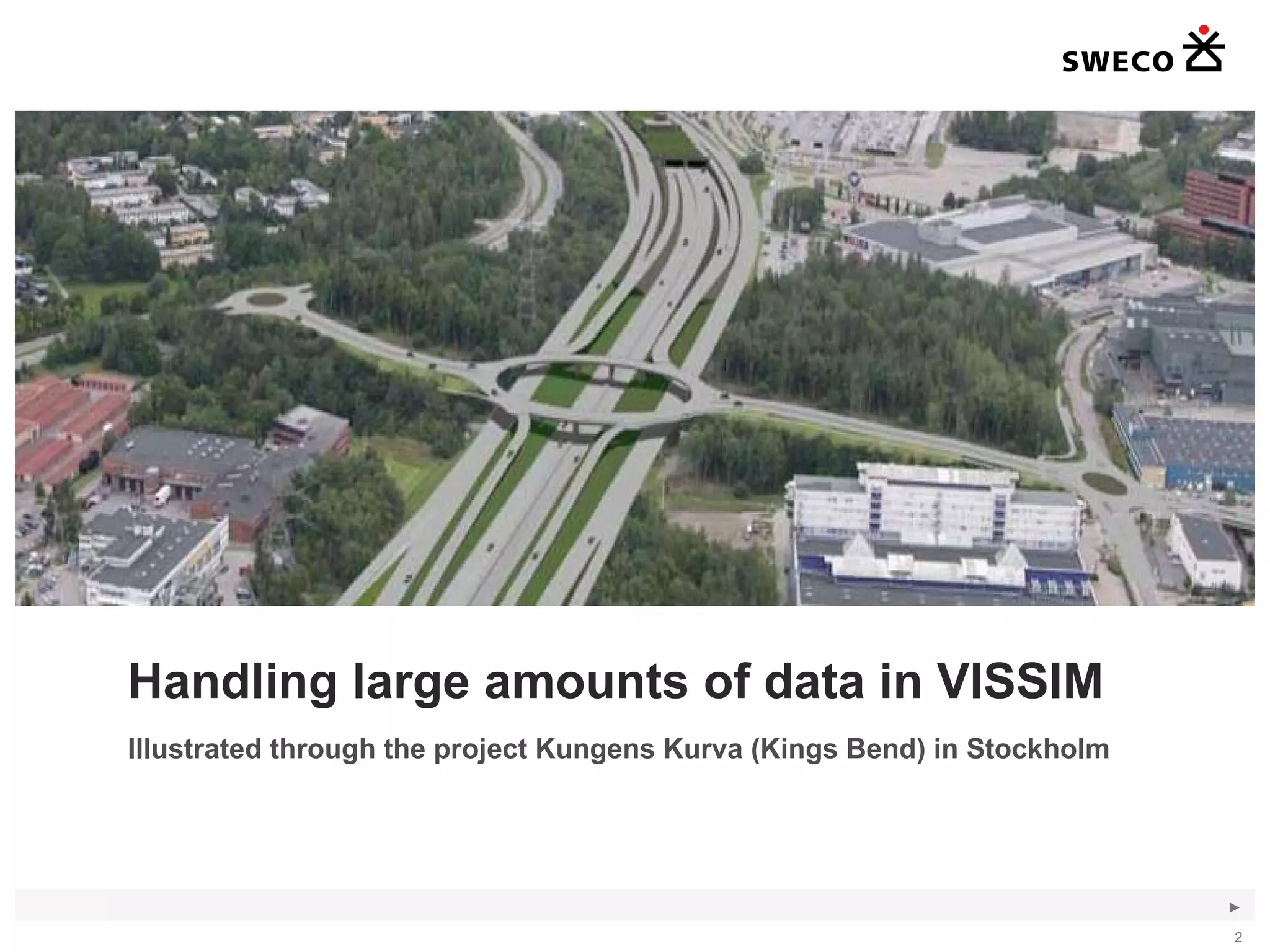
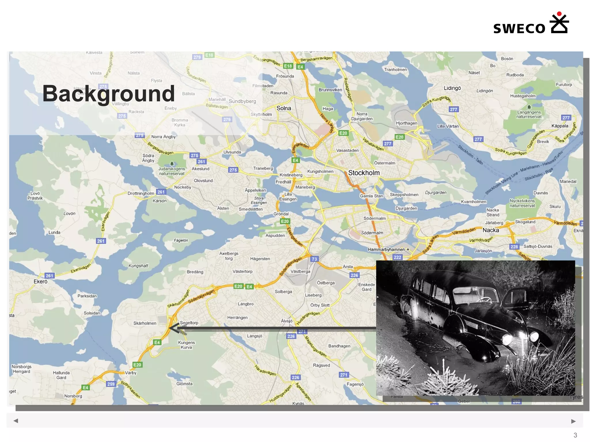
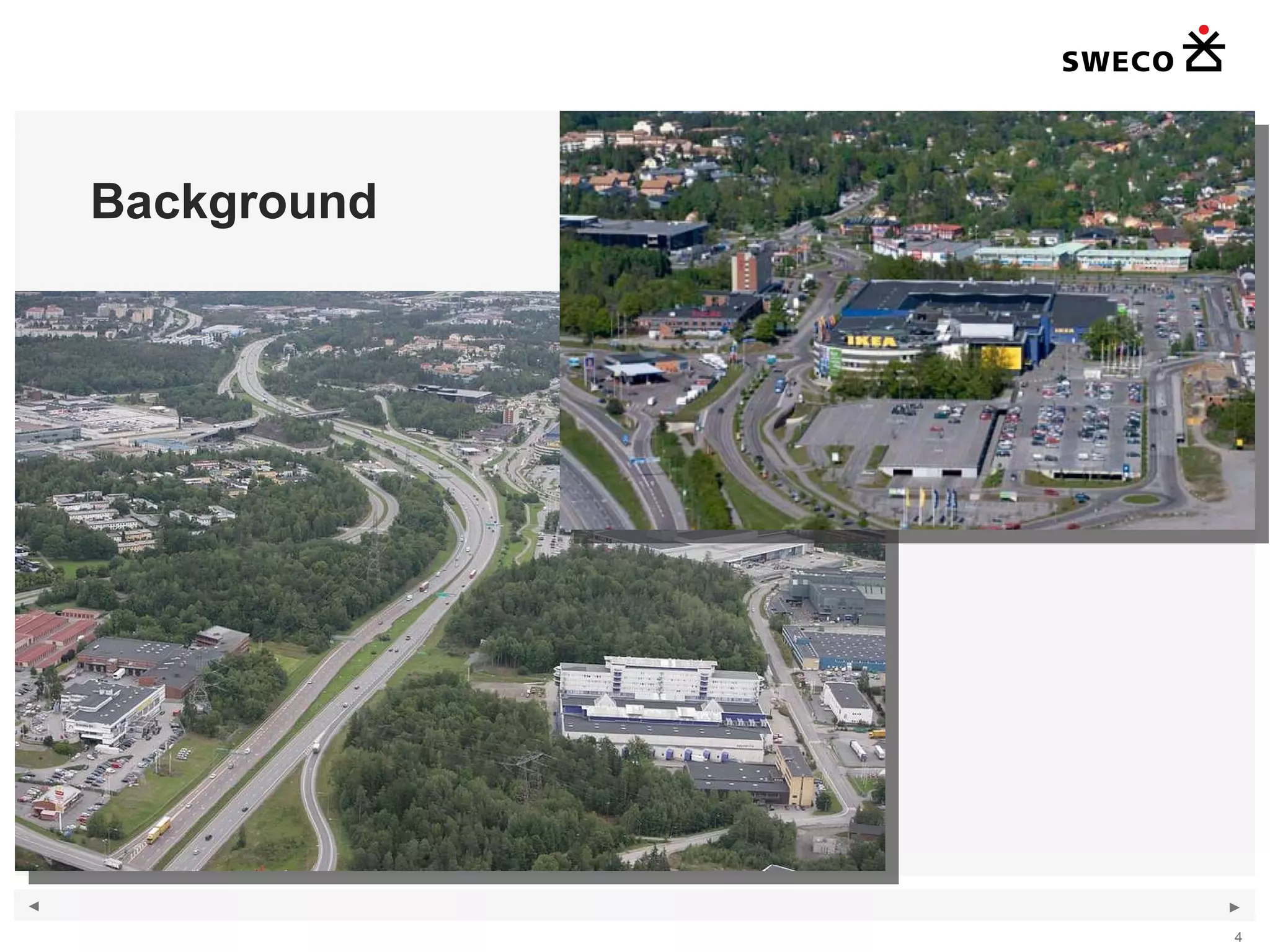
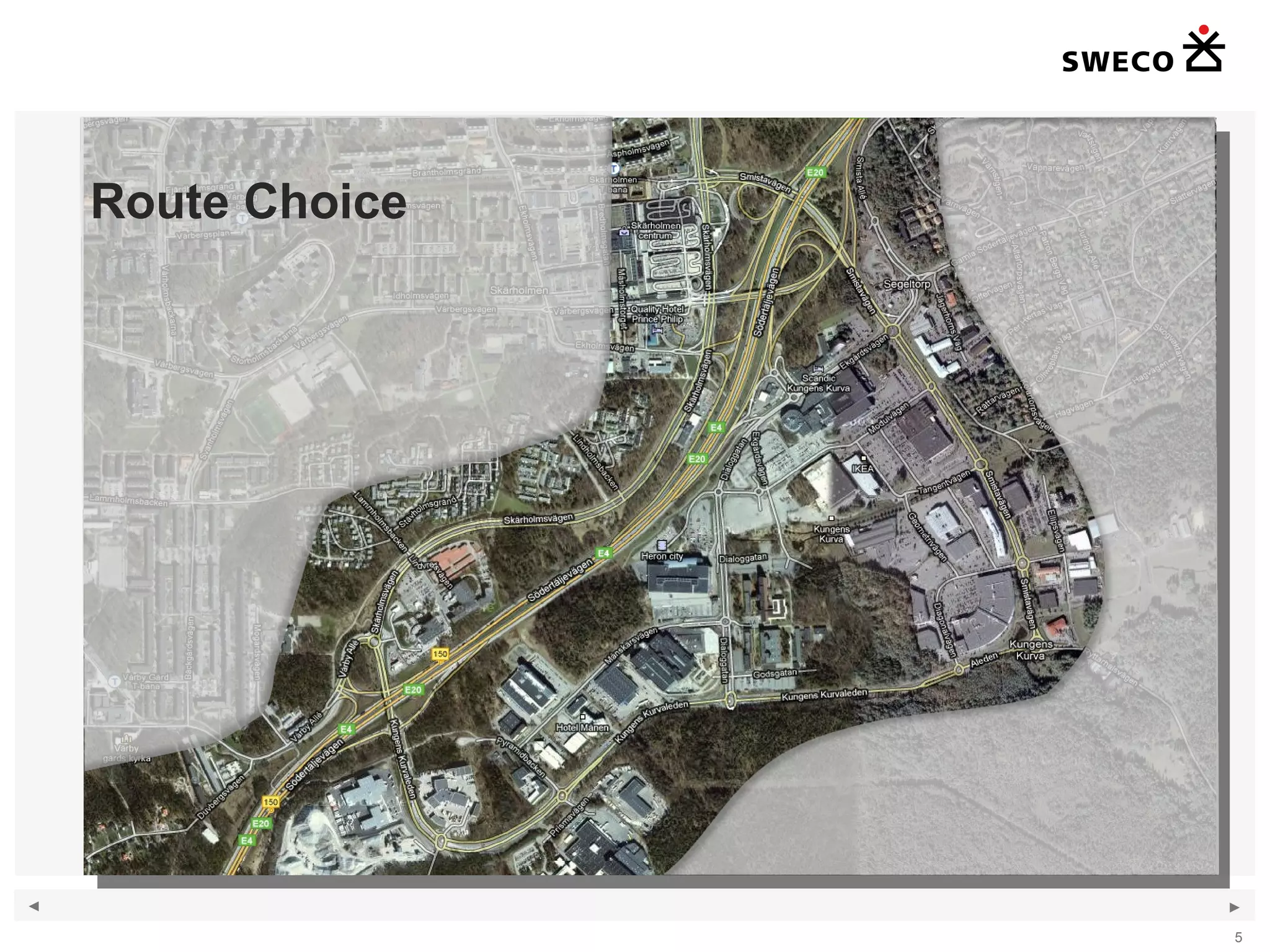
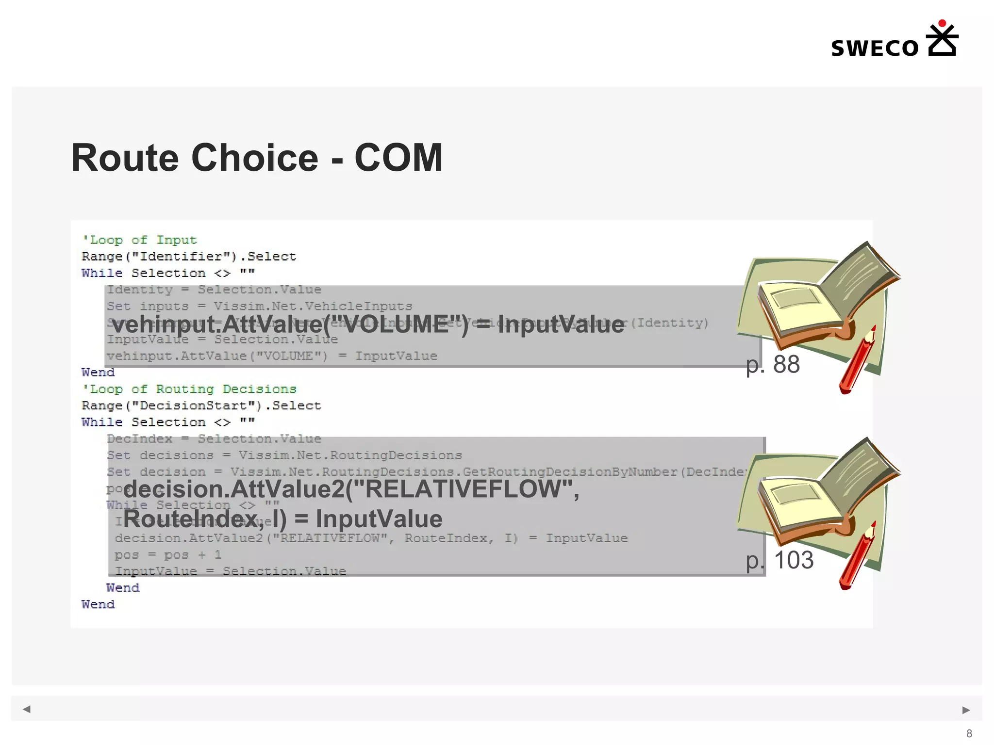
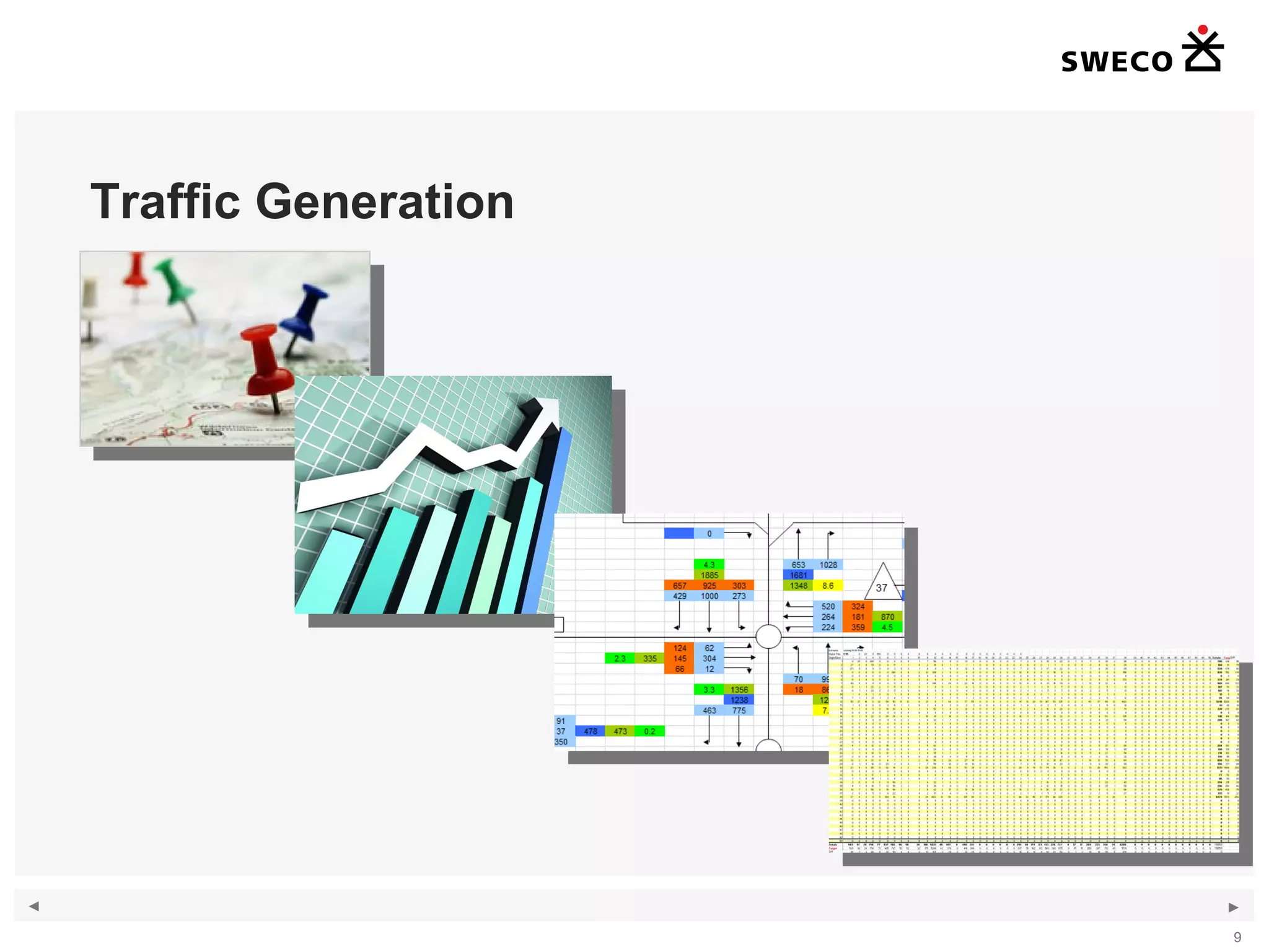


1) The document discusses handling large amounts of data in the traffic simulation software VISSIM through the example project of Kungens Kurva in Stockholm. 2) It covers topics such as route choice modeling, traffic generation, mapping counts, matrix development using the Furness method, and validating the VISSIM model. 3) The document provides guidance on modeling route choices, inputting traffic volumes, developing origin-destination matrices that match traffic counts, and addressing challenges in validating large-scale VISSIM models.