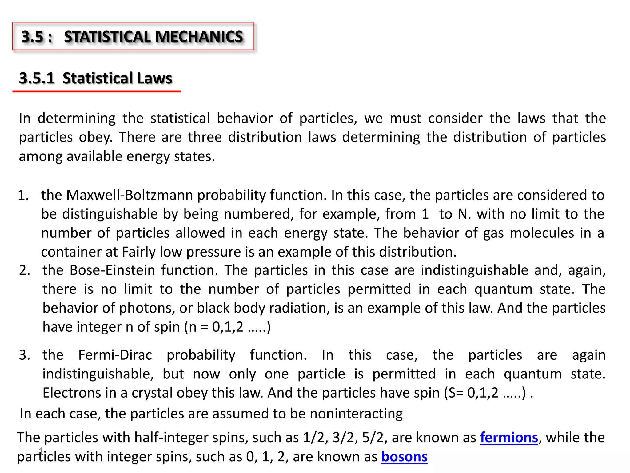
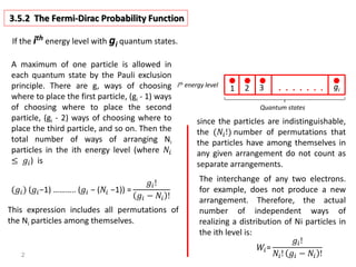
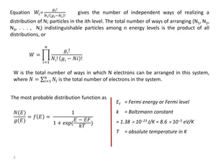
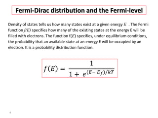
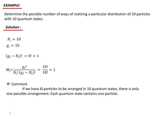
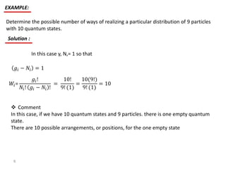
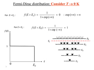
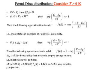
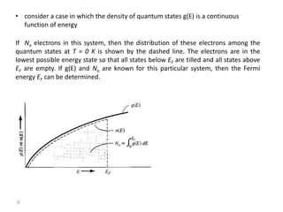
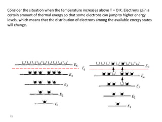
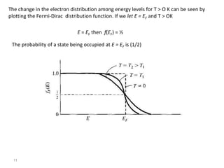
The document discusses statistical mechanics, focusing on three distribution laws: Maxwell-Boltzmann, Bose-Einstein, and Fermi-Dirac. It explains how these functions describe the behavior of distinguishable and indistinguishable particles in various energy states and includes formulas for calculating particle distributions and probabilities. Additionally, it covers the effects of temperature on electron distribution and introduces the Boltzmann approximation to the Fermi-Dirac function.

1. 3.5 : STATISTICAL MECHANICS
3.5.1 Statistical Laws
In determining the statistical behavior of particles, we must consider the laws that the
particles obey. There are three distribution laws determining the distribution of particles
among available energy states.
1. the Maxwell-Boltzmann probability function. In this case, the particles are considered to
be distinguishable by being numbered, for example, from 1 to N. with no limit to the
number of particles allowed in each energy state. The behavior of gas molecules in a
container at Fairly low pressure is an example of this distribution.
2. the Bose-Einstein function. The particles in this case are indistinguishable and, again,
there is no limit to the number of particles permitted in each quantum state. The
behavior of photons, or black body radiation, is an example of this law. And the particles
have integer n of spin (n = 0,1,2 …..)
3. the Fermi-Dirac probability function. In this case, the particles are again
indistinguishable, but now only one particle is permitted in each quantum state.
Electrons in a crystal obey this law. And the particles have spin (S= 0,1,2 …..) .
In each case, the particles are assumed to be noninteracting
The particles with half-integer spins, such as 1/2, 3/2, 5/2, are known as fermions, while the
particles with integer spins, such as 0, 1, 2, are known as bosons1

2. 3.5.2 The Fermi-Dirac Probability Function
ith energy level
Quantum states
1 2 3 gi
If the ith energy level with gi quantum states.
A maximum of one particle is allowed in
each quantum state by the Pauli exclusion
principle. There are g, ways of choosing
where to place the first particle, (gi - 1) ways
of choosing where to place the second
particle, (gi - 2) ways of choosing where to
place the third particle, and so on. Then the
total number of ways of arranging Ni
particles in the ith energy level (where 𝑁𝑖
≤ 𝑔𝑖) is
(𝑔𝑖) (𝑔𝑖−1) ……….. (𝑔𝑖 − (𝑁𝑖 −1)) =
𝑔𝑖!
𝑔𝑖 − 𝑁𝑖 !
This expression includes all permutations of
the Ni particles among themselves.
since the particles are indistinguishable,
the (𝑁𝑖!) number of permutations that
the particles have among themselves in
any given arrangement do not count as
separate arrangements.
The interchange of any two electrons.
for example, does not produce a new
arrangement. Therefore, the actual
number of independent ways of
realizing a distribution of Ni particles in
the ith level is:
𝑊𝑖=
𝑔𝑖!
𝑁𝑖! 𝑔𝑖 − 𝑁𝑖 !2

3. Equation 𝑊𝑖=
𝑔𝑖!
𝑁 𝑖! 𝑔𝑖−𝑁 𝑖 !
gives the number of independent ways of realizing a
distribution of N; particles in the ith level. The total number of ways of arranging (N1, N2,
N3, . . . , Ni) indistinguishable particles among n energy levels is the product of all
distributions, or
𝑊 =
𝑖=1
𝑛
𝑔𝑖!
𝑁𝑖! 𝑔𝑖 − 𝑁𝑖 !
W is the total number of ways in which N electrons can be arranged in this system,
where 𝑁 = 𝑖=1
𝑛
𝑁𝑖 is the total number of electrons in the system.
The most probable distribution function as
𝑁(𝐸)
𝑔(𝐸)
= 𝑓 𝐸 =
1
1 + exp(
𝐸 − 𝐸𝐹
𝑘𝑇
)
EF = Fermi energy or Fermi level
k = Boltzmann constant
= 1.38 1023 J/K = 8.6  105 eV/K
T = absolute temperature in K
3

4. Fermi-Dirac distribution and the Fermi-level
Density of states tells us how many states exist at a given energy E . The Fermi
function f(E) specifies how many of the existing states at the energy E will be
filled with electrons. The function f(E) specifies, under equilibrium conditions,
the probability that an available state at an energy E will be occupied by an
electron. It is a probability distribution function.
𝑓 𝐸 =
1
1 + 𝑒(𝐸− 𝐸 𝑓)/𝑘𝑇
4

5. EXAMPLE:
Determine the possible number of ways of realizing a particular distribution of 10 particles
with 10 quantum states.
Solution :
𝑔𝑖 = 10
𝑁𝑖 = 10
𝑊𝑖=
𝑔𝑖!
𝑁𝑖! 𝑔𝑖 − 𝑁𝑖 !
=
10!
10!
= 1
𝑔𝑖 − 𝑁𝑖 ! = 0! = 1
 Comment
If we have I0 particles to be arranged in 10 quantum states, there is only
one possible arrangement. Each quantum state contains one particle.
5

6. EXAMPLE:
Determine the possible number of ways of realizing a particular distribution of 9 particles
with 10 quantum states.
Solution :
In this case y, N,= 1 so that
𝑔𝑖 − 𝑁𝑖 = 1
𝑊𝑖=
𝑔𝑖!
𝑁𝑖! 𝑔𝑖 − 𝑁𝑖 !
=
10!
9! (1)
=
10(9!)
9! (1)
= 10
 Comment
In this case, if we have 10 quantum states and 9 particles. there is one empty quantum
state.
There are 10 possible arrangements, or positions, for the one empty state
6

7. Fermi-Dirac distribution: Consider T  0 K
For E < EF :


 )(exp:0
)(exp1
1
)( FEEf
1
)(exp1
1
)( F 

 EEf
EF
0
f (E)
1
E
For E > EF :
Ef
7

8. • If E = EF then f(EF) = ½
• If then
Thus the following approximation is valid:
i.e., most states at energies 3kT above EF are empty.
• If then
Thus the following approximation is valid:
So, 1f(E) = Probability that a state is empty, decays to zero.
So, most states will be filled.
kT (at 300 K) = 0.025eV, Eg(Si) = 1.1eV, so 3kT is very small in
comparison.
kTEE 3F  1exp F 




 
kT
EE





 

kT
EE
Ef
)(
exp)( F
kTEE 3F  1exp F 




 
kT
EE





 

kT
EE
Ef Fexp1)(
Fermi-Dirac distribution: Consider T > 0 K
8

9. • consider a case in which the density of quantum states g(E) is a continuous
function of energy
If No electrons in this system, then the distribution of these electrons among the
quantum states at T = 0 K is shown by the dashed line. The electrons are in the
lowest possible energy state so that all states below EF are tilled and all states above
EF are empty. If g(E) and No are known for this particular system, then the Fermi
energy EF can be determined.
9

10. Consider the situation when the temperature increases above T = O K. Electrons gain a
certain amount of thermal energy so that some electrons can jump to higher energy
levels, which means that the distribution of electrons among the available energy states
will change.
Ef
10

11. The change in the electron distribution among energy levels for T > O K can be seen by
plotting the Fermi-Dirac distribution function. If we let E = EF and T > OK
E = EF then f(EF) = ½
The probability of a state being occupied at E = EF is (1/2)
11

12. Determine the probability that an energy level 3kT above the Fermi energy is occupied
by an electron.
EXAMPLE:
Solution :
𝑓 𝐸 =
1
1 + 𝑒(𝐸− 𝐸 𝑓)/𝑘𝑇
=
1
1 + 𝑒3𝑘𝑇/𝑘𝑇
= 0.0474
H.W : E3.4 , E3.5 , E3.6 and E3.7 P. s 93 and 94
the probability of a state a distance dE above Ef
occupied is the same as the probability of a
state a distance dE below EF empty. The
function fr (E) is symmetrical with the function
(1 - ff(E) about t Fermi energy, EF
12

13. Consider the case when E - EF >> kT . where the exponential term in the denominator of
Equation 𝑓 𝐸 =
1
1+ 𝑒
(𝐸− 𝐸 𝑓)/𝑘𝑇 is much greater than unity. We may neglect the I in the
denominator, so the Femi-Dirac dihtribution function becomes
𝑓 𝐸 ≈ 𝑒−(𝐸− 𝐸 𝑓)/𝑘𝑇
This equation is known as the Maxwell - Bolumann approximation, or simply the Boltzmann
approximation to the Fermi-Dirac distribution function.
This figure gives an indication of the range
of energies over which the approximation
is valid.
13

14. To determine the energy at which the Bolt7mann approximation may be considered valid.
Calculate the energy, in terms of 𝑘𝑇 and 𝐸 𝐹 . at which the difference between the
Boltzmann approximation and the Fermi-Dirac function is 5 percent of the Fermi function.
EXAMPLE:
Solution :
exp −(𝐸− 𝐸 𝑓)/𝑘𝑇 −
1
1+exp (𝐸− 𝐸 𝑓)/𝑘𝑇
1
1+exp (𝐸− 𝐸 𝑓)/𝑘𝑇
= 0.05
exp −(𝐸 − 𝐸𝑓)/𝑘𝑇 . 1 + exp
𝐸− 𝐸 𝑓
𝑘𝑇
− 1 = 0.05
exp −(𝐸 − 𝐸𝑓)/𝑘𝑇 = 0.05
𝐸 − 𝐸𝑓 = 𝑘𝑇𝑙𝑛
1
0.05
≈ 3𝑘𝑇
H.W : Solve the odd problems of ch.3
14

15. Equilibrium distribution of carriers
Distribution of carriers = DOS probability of occupancy
= g (E) f (E)
(where DOS = Density of states)
Total number of electrons in CB (conduction band) =
 top
C
d)()(C0
E
E
EEfEgn
Total number of holes in VB (valence band) =
   V
Bottom
d)(1)(V0
E
E
EEfEgp
15