Download to read offline

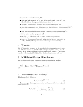
![6 Preliminary results for UCF-Sports Dataset
The following results are obtained without tuning the MRF objective functions
parameters: σs and σd. The evaluation is performed for localization of action
in the video sequences.
Method mAP
Raptis et al [2011] 79.4%
Lan at al [2012] 73.1 %
SDPM [2011] 75.2 %
Ma et al [2013] 81.7 %
Xu et al [2014] 78.8 %
Ours 77.5 %
4](https://image.slidesharecdn.com/segmentationbasedgraphconstruction5-150601160506-lva1-app6892/85/Segmentation-based-graph-construction-5-4-320.jpg)

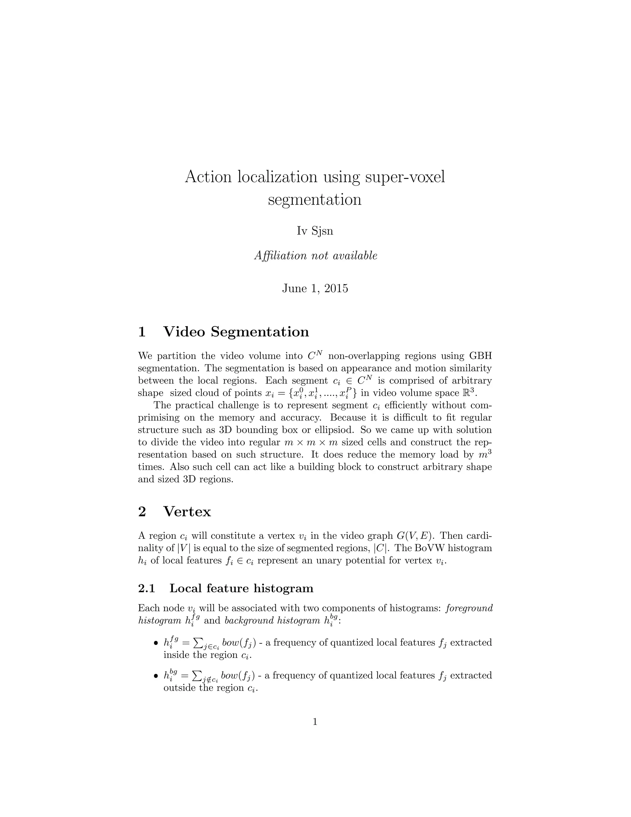
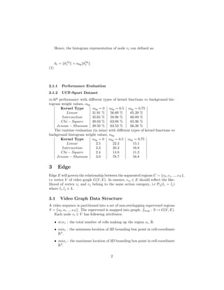
The document proposes a method for action localization in videos using supervoxel segmentation and modeling the video as a graph. It segments the video into irregularly shaped regions, constructs graph vertices from the regions, and graph edges to capture relationships between regions. Histograms of local features are used to represent vertices. A classifier is trained on the vertices to label actions, and an MRF model is optimized to jointly infer region labels for localization. Preliminary results on the UCF Sports dataset achieve 77.5% mAP for action localization.


![[Review] BoxInst: High-Performance Instance Segmentation with Box Annotations...](https://cdn.slidesharecdn.com/ss_thumbnails/boxinstreviewcdm-210627063153-thumbnail.jpg?width=640&height=640&fit=bounds)