This document discusses various types of mechanical vibrations including undamped, underdamped, critically damped, and overdamped motion. It provides examples of solving differential equations describing simple harmonic motion under different damping conditions and applying the solutions to problems involving springs, pendulums, and other oscillating systems. Specific cases are worked through to determine characteristics like frequency, period, and damping behavior.
![SECTION 5.4
Mechanical Vibrations
In this section we discuss four types of free motion of a mass on a spring — undamped,
underdamped, critically damped, and overdamped. However, the undamped and underdamped
cases — in which actual oscillations occur — are emphasized because they are both the most
interesting and the most important cases for applications.
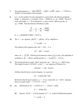
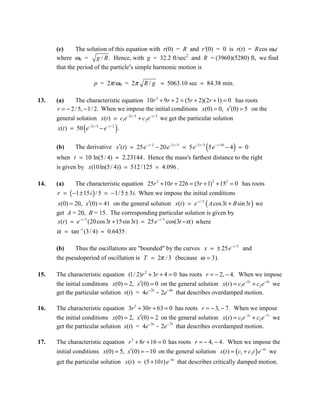
1. Frequency: ω 0 = k / m = 16 / 4 = 2 rad / sec = 1/ π Hz
Period: P = 2π / ω 0 = 2π / 2 = π sec
2. Frequency ω 0 = k / m = 48 / 0.75 = 8 rad / sec = 4 / π Hz
Period: P = 2π / ω 0 = 2π / 8 = π / 4 sec
3. The spring constant is k = 15 N/0.20 m = 75 N/m. The solution of 3x″ + 75x = 0
with x(0) = 0 and x′(0) = -10 is x(t) = -2 sin 5t. Thus the amplitude is 2 m; the
frequency is ω 0 = k / m = 75 / 3 = 5 rad / sec = 2.5 / π Hz ; and the period is 2π/5 sec.
4. (a) With m = 1/4 kg and k = (9 N)/(0.25 m) = 36 N/m we find that ω0 = 12
rad/sec. The solution of x″ + 144x = 0 with x(0) = 1 and x′(0) = -5 is
x(t) = cos 12t - (5/12)sin 12t
= (13/12)[(12/13)cos 12t - (5/13)sin 12t]
x(t) = (13/12)cos(12t - α)
where α = 2π - tan-1(5/12) ≈ 5.8884.
(b) C = 13/12 ≈ 1.0833 ft and T = 2π/12 ≈ 0.5236 sec.
5. The gravitational acceleration at distance R from the center of the earth is g = GM/R2.
According to Equation (6) in the text the (circular) frequency ω of a pendulum is given
by ω2 = g/L = GM/R2L, so its period is p = 2π/ω = 2πR L / GM .
6. If the pendulum in the clock executes n cycles per day (86400 sec) at Paris, then its
period is p1 = 86400/n sec. At the equatorial location it takes 24 hr 2 min 40 sec =
86560 sec for the same number of cycles, so its period there is p2 = 86560/n sec. Now
let R1 = 3956 mi be the Earth′s "radius" at Paris, and R2 its "radius" at the equator.
Then substitution in the equation p1 /p2 = R1 /R2 of Problem 5 (with L1 = L2) yields
R2 = 3963.33 mi. Thus this (rather simplistic) calculation gives 7.33 mi as the thickness
of the Earth's equatorial bulge.](https://image.slidesharecdn.com/sect5-4-100319104203-phpapp02/85/Sect5-4-1-320.jpg)
![SECTION 5.4
Mechanical Vibrations
In this section we discuss four types of free motion of a mass on a spring — undamped,
underdamped, critically damped, and overdamped. However, the undamped and underdamped
cases — in which actual oscillations occur — are emphasized because they are both the most
interesting and the most important cases for applications.
1. Frequency: ω 0 = k / m = 16 / 4 = 2 rad / sec = 1/ π Hz
Period: P = 2π / ω 0 = 2π / 2 = π sec
2. Frequency ω 0 = k / m = 48 / 0.75 = 8 rad / sec = 4 / π Hz
Period: P = 2π / ω 0 = 2π / 8 = π / 4 sec
3. The spring constant is k = 15 N/0.20 m = 75 N/m. The solution of 3x″ + 75x = 0
with x(0) = 0 and x′(0) = -10 is x(t) = -2 sin 5t. Thus the amplitude is 2 m; the
frequency is ω 0 = k / m = 75 / 3 = 5 rad / sec = 2.5 / π Hz ; and the period is 2π/5 sec.
4. (a) With m = 1/4 kg and k = (9 N)/(0.25 m) = 36 N/m we find that ω0 = 12
rad/sec. The solution of x″ + 144x = 0 with x(0) = 1 and x′(0) = -5 is
x(t) = cos 12t - (5/12)sin 12t
= (13/12)[(12/13)cos 12t - (5/13)sin 12t]
x(t) = (13/12)cos(12t - α)
where α = 2π - tan-1(5/12) ≈ 5.8884.
(b) C = 13/12 ≈ 1.0833 ft and T = 2π/12 ≈ 0.5236 sec.
5. The gravitational acceleration at distance R from the center of the earth is g = GM/R2.
According to Equation (6) in the text the (circular) frequency ω of a pendulum is given
by ω2 = g/L = GM/R2L, so its period is p = 2π/ω = 2πR L / GM .
6. If the pendulum in the clock executes n cycles per day (86400 sec) at Paris, then its
period is p1 = 86400/n sec. At the equatorial location it takes 24 hr 2 min 40 sec =
86560 sec for the same number of cycles, so its period there is p2 = 86560/n sec. Now
let R1 = 3956 mi be the Earth′s "radius" at Paris, and R2 its "radius" at the equator.
Then substitution in the equation p1 /p2 = R1 /R2 of Problem 5 (with L1 = L2) yields
R2 = 3963.33 mi. Thus this (rather simplistic) calculation gives 7.33 mi as the thickness
of the Earth's equatorial bulge.](https://image.slidesharecdn.com/sect5-4-100319104203-phpapp02/75/Sect5-4-1-2048.jpg)
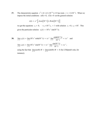
![18. The characteristic equation 2r 2 + 12r + 50 = 0 has roots r = − 3 ± 4 i. When we impose
the initial conditions x(0) = 0, x′(0) = − 8 on the general solution
x(t ) = e−3t ( A cos 4t + B sin 4t ) we get the particular solution
x(t ) = − 2 e −3t sin 4t = 2 e −3t cos(4t − π / 2) that describes underdamped motion.
19. The characteristic equation 4r 2 + 20r + 169 = 0 has roots r = − 5 / 2 ± 6 i. When we
impose the initial conditions x(0) = 4, x′(0) = 16 on the general solution
x(t ) = e−5 t / 2 ( A cos 6t + B sin 6t ) we get the particular solution
x(t) = e-5t/2 [4 cos 6t + (13/3) sin 2t] ≈ (1/3) 313 e-5t/2 cos(6t - 0.8254)
that describes underdamped motion.
20. The characteristic equation 2r 2 + 16r + 40 = 0 has roots r = − 4 ± 2 i. When we impose
the initial conditions x(0) = 5, x′(0) = 4 on the general solution
x(t ) = e−4 t ( A cos 2t + B sin 4t ) we get the particular solution
x(t) = e-4t (5 cos 2t + 12 sin 2t) ≈ 13 e-4t cos(2t - 1.1760)
that describes underdamped motion.
21. The characteristic equation r 2 + 10r + 125 = 0 has roots r = − 5 ± 10 i. When we impose
the initial conditions x(0) = 6, x′(0) = 50 on the general solution
x(t ) = e−5 t ( A cos10t + B sin10t ) we get the particular solution
x(t) = e-5t (6 cos 10t + 8 sin 10t) ≈ 10 e-5t cos(10t - 0.9273)
that describes underdamped motion.
22. (a) With m = 12/32 = 3/8 slug, c = 3 lb-sec/ft, and k = 24 lb/ft, the differential
equation is equivalent to 3x″ + 24x′ + 192x = 0. The characteristic equation
3r 2 + 24r + 192 = 0 has roots r = − 4 ± 4 3 i. When we impose the initial conditions
( )
x(0) = 1, x′(0) = 0 on the general solution x(t ) = e−4 t A cos 4t 3 + B sin 4t 3 we get
the particular solution
x(t) = e-4t [cos 4t 3 + (1/ 3 )sin 4t 3 ]
= (2/ 3 )e-4t [( 3 /2)cos 4t 3 + (1/2)sin 4t 3 ]
x(t) = (2/ 3 )e-4t cos(4t 3 – π / 6 ).](https://image.slidesharecdn.com/sect5-4-100319104203-phpapp02/85/Sect5-4-4-320.jpg)
![(b) The time-varying amplitude is 2/ 3 ≈ 1.15 ft; the frequency is 4 3 ≈ 6.93
rad/sec; and the phase angle is π / 6 .
23. (a) With m = 100 slugs we get ω = k /100 . But we are given that
ω = (80 cycles/min)(2π)(1 min/60 sec) = 8π/3,
and equating the two values yields k ≈ 7018 lb/ft.
(b) With ω1 = 2π(78/60) sec-1, Equation (21) in the text yields c ≈ 372.31
lb/(ft/sec). Hence p = c/2m ≈ 1.8615. Finally e-pt = 0.01 gives t ≈ 2.47 sec.
30. In the underdamped case we have
x(t) = e-pt [A cos ω1t + B sin ω1t],
x′(t) = -pept [A cos ω1t + B sin ω1t] + e-pt [-Aω1sin ω1t + Bω1cos ω1t].
The conditions x(0) = x0, x′(0) = v0 yield the equations A = x0 and
-pA + Bω1 = v0, whence B = (v0 + px0)/ ω1.
31. The binomial series
α (α − 1) 2 α (α − 1)(α − 2) 3
(1 + x )
α
= 1+α x + x + x +
2! 3!
converges if x 1. (See, for instance, Section 11.8 of Edwards and Penney, Calculus
with Analytic Geometry, 5th edition, Prentice Hall, 1998.) With α = 1/ 2 and
x = − c 2 / 4mk in Eq. (21) of Section 5.4 in this text, the binomial series gives
k c2 k c2
ω1 = ω0 − p 2 =
2
− = 1−
m 4m 2 m 4 mk
k c2 c4 c2
= 1− − 2 2
− ≈ ω 0 1 − .
m 8mk 128m k 8mk
32. If x(t) = Ce-pt cos(ω1t - α) then
x′(t) = -pCe-pt cos(ω1t - α) + Cω1e-pt sin(ω1t - α) = 0
yields tan(ω1t - α) = -p/ ω1.](https://image.slidesharecdn.com/sect5-4-100319104203-phpapp02/85/Sect5-4-5-320.jpg)
![33. If x1 = x(t1) and x2 = x(t2) are two successive local maxima, then ω1t2 = ω1t1 + 2π
so
x1 = C exp(-pt1) cos(ω1t1 - α),
x2 = C exp(-pt2) cos(ω1t2 - α) = C exp(-pt2) cos(ω1t1 - α).
Hence x1 /x2 = exp[-p(t1 - t2)], and therefore
ln(x1 /x2) = -p(t1 - t2) = 2πp/ ω1.
34. With t1 = 0.34 and t2 = 1.17 we first use the equation ω1t2 = ω1t1 + 2π from
Problem 32 to calculate ω1 = 2π/(0.83) ≈ 7.57 rad/sec. Next, with x1 = 6.73 and
x2 = 1.46, the result of Problem 33 yields
p = (1/0.83) ln(6.73/1.46) ≈ 1.84.
Then Equation (16) in this section gives
c = 2mp = 2(100/32)(1.84) ≈ 11.51 lb-sec/ft,
and finally Equation (21) yields
k = (4m2ω12 + c2)/4m ≈ 189.68 lb/ft.
35. The characteristic equation r 2 + 2r + 1 = 0 has roots r = − 1, − 1. When we impose the
initial conditions x(0) = 0, x′(1) = 0 on the general solution x(t ) = ( c1 + c2t ) e − t we get
the particular solution x1 (t ) = t e − t .
36. The characteristic equation r 2 + 2r + (1 − 10 −2 n ) = 0 has roots r = − 1 ± 10− n. When we
impose the initial conditions x(0) = 0, x′(1) = 0 on the general solution
( ) ( )
x(t ) = c1 exp −1 + 10− n t + c1 exp −1 − 10− n t
we get the equations
c1 + c2 = 0, (−1 + 10 ) c + (−1 − 10 ) c
−n
1
−n
2 = 1
with solution c1 = 2n −15n , c2 = 2 n −15n. This gives the particular solution
exp(10− n t ) − exp( −10− n t )
x2 (t ) = 10n e − t n −t −n
= 10 e sinh(10 t ).
2 ](https://image.slidesharecdn.com/sect5-4-100319104203-phpapp02/85/Sect5-4-6-320.jpg)


![[Vvedensky d.] group_theory,_problems_and_solution(book_fi.org)](https://cdn.slidesharecdn.com/ss_thumbnails/vvedenskyd-grouptheoryproblemsandsolutionbookfi-org-130405071812-phpapp02-thumbnail.jpg?width=640&height=640&fit=bounds)


![Week 8 [compatibility mode]](https://cdn.slidesharecdn.com/ss_thumbnails/week8compatibilitymode-130213163443-phpapp01-thumbnail.jpg?width=640&height=640&fit=bounds)


