Downloaded 101 times


![12
SOLO
Statistical Independent Events
( ) ( ) ( ) ( )
( ) ( ) ( ) ( ) ( )∏∑∏∑∏∑
∑∑∑
=
−
≠≠
=
≠
=
=
=
−
≠≠
≠
==
−+−+−=
−+−+−=
n
i
i
n
n
kji
kji i
i
n
ji
ji i
i
n
i
i
tIndependen
lStatisticaA
n
i
i
n
n
kji
kji
kji
n
ji
ji
ji
n
i
i
n
i
i
AAAA
AAAAAAAA
i
1
1
3
,.
3
1
2
.
2
1
1
1
1
1
3
,.
2
.
1
11
Pr1PrPrPr
Pr1PrPrPrPr
From Theorem of Addition
Therefore
( )[ ]∏==
−=
−
n
i
i
tIndependen
lStatisticaA
n
i
i AA
i
11
Pr1Pr1 ( )[ ]∏==
−−=
n
i
i
tIndependen
lStatisticaA
n
i
i AA
i
11
Pr11Pr
Since OAASAA
n
i
i
n
i
i
n
i
i
n
i
i /=
=
====
1111
&
=
−
==
n
i
i
n
i
i AA
11
PrPr1
( )∏==
=
n
i
i
tIndependen
lStatisticaA
n
i
i AA
i
11
PrPr
If the n events Ai i = 1,2,…n are statistical independent
than are also statistical independentiA
( )∏=
=
n
i
iA
1
Pr
=
=
n
i
i
MorganDe
A
1
Pr ( )[ ]∏=
−=
n
i
i
tIndependen
lStatisticaA
A
i
1
Pr1
( ) nrAA
r
i
i
r
i
i ,,2PrPr
11
=∀=
∏==
Table of Content
Review of Probability](https://image.slidesharecdn.com/3-recursivebayesianestimation-150113075152-conversion-gate02/85/3-recursive-bayesian-estimation-12-320.jpg)
![13
SOLO Review of Probability
Expected Value or Mathematical Expectation
Given a Probability Density Function p (x) we define the Expected Value
For a Continuous Random Variable: ( ) ( )∫
+∞
∞−
= dxxpxxE X:
For a Discrete Random Variable: ( ) ( )∑=
k
kXk xpxxE :
For a general function g (x) of the
Random Variable x: ( )[ ] ( ) ( )∫
+∞
∞−
= dxxpxgxgE X:
( )xp
x
0 ∞+∞−
0.1
( )xE
( )
( )
( )∫
∫
∞+
∞−
+∞
∞−
=
dxxp
dxxpx
xE
X
X
:
The Expected Value is the center of
surface enclosed between the
Probability Density Function and x
axis.
Table of Content](https://image.slidesharecdn.com/3-recursivebayesianestimation-150113075152-conversion-gate02/85/3-recursive-bayesian-estimation-13-320.jpg)
![14
SOLO Review of Probability
Variance
Given a Probability Density Functions p (x) we define the Variance
( ) ( )[ ]{ } ( ) ( )[ ] ( ) ( )22222
2: xExExExExxExExExVar −=+−=−=
Central Moment
( ) { }k
k xEx =:'µ
Given a Probability Density Functions p (x) we define the Central Moment
of order k about the origin
( ) ( )[ ]{ } ( ) ( )∑=
−−
−
=−=
k
j
jk
j
jkk
k xE
j
k
xExEx
0
'1: µµ
Given a Probability Density Functions p (x) we define the Central Moment
of order k about the Mean E (x)
Table of Content](https://image.slidesharecdn.com/3-recursivebayesianestimation-150113075152-conversion-gate02/85/3-recursive-bayesian-estimation-14-320.jpg)
![15
SOLO Review of Probability
Moments
Normal Distribution ( ) ( ) ( )[ ]
σπ
σ
σ
2
2/exp
;
22
x
xpX
−
=
[ ] ( )
−⋅
=
oddnfor
evennforn
xE
n
n
0
131 σ
[ ]
( )
+=
=−⋅
= +
12!2
2
2131
12
knfork
knforn
xE kk
n
n
σ
π
σ
Proof:
Start from: and differentiate k time with respect to a( ) 0exp 2
>=−∫
∞
∞−
a
a
dxxa
π
Substitute a = 1/(2σ2
) to obtain E [xn
]
( ) ( ) 0
2
1231
exp 12
22
>
−⋅
=− +
∞
∞−
∫ a
a
k
dxxax kk
k π
[ ] ( ) ( )[ ] ( ) ( )[ ]
( ) ( ) 12
!
0
122/
0
222221212
!2
2
exp
2
22
2/exp
2
2
2/exp
2
1
2
+
∞+
=
∞∞
∞−
++
=−=
−=−=
∫
∫∫
kk
k
k
k
xy
kkk
kdyyy
xdxxxdxxxxE
σ
πσ
σ
π
σ
σπ
σ
σπ
σ
Now let compute:
[ ] [ ]( )2244
33 xExE == σ
Chi-square](https://image.slidesharecdn.com/3-recursivebayesianestimation-150113075152-conversion-gate02/85/3-recursive-bayesian-estimation-15-320.jpg)

![17
SOLO Review of Probability
Functions of one Random Variable (continue – 1)
Example 1
bxay += ( )
−
=
a
by
p
a
yp XY
1
Example 2
x
a
y = ( )
=
y
a
p
y
a
yp XY 2
Example 3
2
xay = ( ) ( )yU
a
y
p
a
y
p
ya
yp XXY
−+
=
2
1
Example 4
xy = ( ) ( ) ( )[ ] ( )yUypypyp XXY −+=
Table of Content](https://image.slidesharecdn.com/3-recursivebayesianestimation-150113075152-conversion-gate02/85/3-recursive-bayesian-estimation-17-320.jpg)
![18
SOLO Review of Probability
Characteristic Function and Moment-Generating Function
Given a Probability Density Functions pX (x) we define the Characteristic Function or
Moment Generating Function
( ) ( )[ ]
( ) ( ) ( ) ( )
( ) ( )
=
==Φ
∑
∫∫
+∞
∞−
+∞
∞−
x
X
XX
X
discretexxpxj
continuousxxPdxjdxxpxj
xjE
ω
ωω
ωω
exp
expexp
exp:
This is in fact the complex conjugate of the Fourier Transfer of the Probability Density
Function. This function is always defined since the sufficient condition of the existence of a
Fourier Transfer :
Given the Characteristic Function we can find the Probability Density
Functions pX (x) using the Inverse Fourier Transfer:
( )
( )
( ) ∞<== ∫∫
+∞
∞−
≥+∞
∞−
1
0
dxxpdxxp X
xp
X
( ) ( ) ( )∫
+∞
∞−
Φ−= ωωω
π
dxjxp XX exp
2
1
is always fulfilled.](https://image.slidesharecdn.com/3-recursivebayesianestimation-150113075152-conversion-gate02/85/3-recursive-bayesian-estimation-18-320.jpg)


![21
SOLO Review of Probability
Probability Distribution and Probability Density Functions (Examples)
(2) Poisson’s Distribution ( ) ( )0
0
exp
!
, k
k
k
nkp
k
−≈
(1) Binomial (Bernoulli) ( )
( )
( ) ( ) knkknk
pp
k
n
pp
knk
n
nkp
−−
−
=−
−
= 11
!!
!
,
0 1 2 3 4 5 6 7 8 9 10 11 12 13 14 k
( )nkP ,
(3) Normal (Gaussian)
( ) ( ) ( )[ ]
σπ
σµ
σµ
2
2/exp
,;
22
−−
=
x
xp
(4) Laplacian Distribution ( )
−
−=
b
x
b
bxp
µ
µ exp
2
1
,;](https://image.slidesharecdn.com/3-recursivebayesianestimation-150113075152-conversion-gate02/85/3-recursive-bayesian-estimation-21-320.jpg)

![23
SOLO Review of Probability
Probability Distribution and Probability Density Functions (Examples)
SOLO
(8) Exponential Distribution
( )
( )
<
≥−
=
00
0exp
;
x
xx
xp
λλ
λ
(9) Chi-square Distribution
( )
( )
( )
( )
<
≥−
Γ=
−
00
02/exp
2/
2/1
;
12/
2/
x
xxx
kkxp
k
k
Γ is the gamma function ( ) ( )∫
∞
−
−=Γ
0
1
exp dttta a
(10) Student’s t-Distribution
( ) ( )[ ]
( ) ( )( ) 2/12
/12/
2/1
; +
+Γ
+Γ
= ν
ννπν
ν
ν
x
xp](https://image.slidesharecdn.com/3-recursivebayesianestimation-150113075152-conversion-gate02/85/3-recursive-bayesian-estimation-23-320.jpg)


![26
SOLO Review of Probability
Normal (Gaussian) Distribution
Karl Friederich Gauss
1777-1855
( )
( )
( )σµ
σπ
σ
µ
σµ ,;:
2
2
exp
,;
2
2
x
x
xp N=
−
−
=
( ) ( )
∫
∞−
−
−=
x
du
u
xP 2
2
2
exp
2
1
,;
σ
µ
σπ
σµ
( ) µ=xE
( ) σ=xVar
( ) ( )[ ]
( ) ( )
−=
−
−=
=Φ
∫
∞+
∞−
2
exp
exp
2
exp
2
1
exp
22
2
2
σω
µω
ω
σ
µ
σπ
ωω
j
duuj
u
xjE
Probability Density Functions
Cumulative Distribution Function
Mean Value
Variance
Moment Generating Function](https://image.slidesharecdn.com/3-recursivebayesianestimation-150113075152-conversion-gate02/85/3-recursive-bayesian-estimation-26-320.jpg)
![27
SOLO Review of Probability
Moments
Normal Distribution ( ) ( ) ( )[ ] ( )σ
σπ
σ
σ ,0;:
2
2/exp
,0;
22
x
x
xpX N=
−
=
[ ] ( )
−⋅
=
oddnfor
evennforn
xE
n
n
0
131 σ
[ ]
( )
+=
=−⋅
= +
12!2
2
2131
12
knfork
knforn
xE kk
n
n
σ
π
σ
Proof:
Start from: and differentiate k time with respect to a( ) 0exp 2
>=−∫
∞
∞−
a
a
dxxa
π
Substitute a = 1/(2σ2
) to obtain E [xn
]
( ) ( ) 0
2
1231
exp 12
22
>
−⋅
=− +
∞
∞−
∫ a
a
k
dxxax kk
k π
[ ] ( ) ( )[ ] ( ) ( )[ ]
( ) ( ) 12
!
0
122/
0
222221212
!2
2
exp
2
22
2/exp
2
2
2/exp
2
1
2
+
∞+
=
∞∞
∞−
++
=−=
−=−=
∫
∫∫
kk
k
k
k
xy
kkk
kdyyy
xdxxxdxxxxE
σ
πσ
σ
π
σ
σπ
σ
σπ
σ
Now let compute:
[ ] [ ]( )2244
33 xExE == σ
Chi-square](https://image.slidesharecdn.com/3-recursivebayesianestimation-150113075152-conversion-gate02/85/3-recursive-bayesian-estimation-27-320.jpg)
![28
SOLO Review of Probability
Normal (Gaussian) Distribution (continue – 1)
Karl Friederich Gauss
1777-1855
( ) ( ) ( ) ( )PxxxxPxxPPxxp
T
,;:
2
1
exp2,; 12/1
N=
−−−= −−
π
A Vector – Valued Gaussian Random Variable has the
Probability Density Functions
where
{ }xEx
= Mean Value
( )( ){ }T
xxxxEP
−−= Covariance Matrix
If P is diagonal P = diag [σ1
2
σ2
2
… σk
2
] then the components of the random vector
are uncorrelated, and
x
( )
( ) ( ) ( ) ( )
∏=
−
−
−
−
=
−
−
−
−
−
−
=
−
−
−
−
−
−
−=
k
i i
i
ii
k
k
kk
kk
k
T
kk
xxxxxxxx
xx
xx
xx
xx
xx
xx
PPxxp
1
2
2
2
2
2
2
2
2
22
1
2
1
2
11
22
11
1
2
2
2
2
1
22
11
2/1
2
2
exp
2
2
exp
2
2
exp
2
2
exp
0
0
2
1
exp2,;
σπ
σ
σπ
σ
σπ
σ
σπ
σ
σ
σ
σ
π
therefore the
components of the
random vector are
also independent](https://image.slidesharecdn.com/3-recursivebayesianestimation-150113075152-conversion-gate02/85/3-recursive-bayesian-estimation-28-320.jpg)


![3131
SOLO Review of Probability
The Law of Large Numbers
Proof of the Weak Law of Large Numbers
( ) iXE i ∀= µ ( ) iXVar i ∀= 2
σ ( )( )[ ] jiXXE ji ≠∀=−− 0µµ
( ) ( ) ( )[ ] µµ ==++= nnnXEXEXE nn //1
( ) ( )[ ]{ } ( ) ( )
( )( )[ ] ( )[ ] ( )[ ]
nn
n
n
XEXE
n
XX
E
n
XX
EXEXEXVar
n
jiXXE
nn
nnn
ji 2
2
2
2
22
1
0
2
1
2
12
σσµµ
µµ
µ
µµ
==
−++−
=
−++−
=
−
++
=−=
≠∀=−−
Given
we have:
Using Chebyshev’s inequality on we obtain:nX ( ) 2
2
/
Pr
ε
σ
εµ
n
Xn ≤≥−
Using this equation we obtain:
( ) ( ) ( ) n
XXX nnn 2
2
1Pr1Pr1Pr
ε
σ
εµεµεµ −≥≥−−≥>−−=≤−
As n approaches infinity, the expression approaches 1.
Chebyshev’s
inequality
q.e.d.
Monte Carlo
Integration
Monte Carlo
Integration
Table of Content](https://image.slidesharecdn.com/3-recursivebayesianestimation-150113075152-conversion-gate02/85/3-recursive-bayesian-estimation-31-320.jpg)

![3333
SOLO Review of Probability
Central Limit Theorem (continue – 1)
Let X1, X2, …, Xm be a sequence of independent random variables with the same
probability distribution function pX (x). Define the statistical mean:
m
XXX
X m
m
+++
=
21
( ) ( ) ( ) ( ) µ=
+++
=
m
XEXEXE
XE m
m
21
( ) ( )[ ]{ } ( ) ( ) ( )
mm
m
m
XXX
EXEXEXVar m
mmmXm
2
2
22
21
22 σσµµµ
σ ==
−++−+−
=−==
Define also the new random variable
( ) ( ) ( ) ( )
m
XXXXEX
Y m
X
mm
m
σ
µµµ
σ
−++−+−
=
−
=
21
:
We have:
The probability distribution of Y tends to become gaussian (normal) as m
tends to infinity, regardless of the probability distribution of the random
variable, as long as the mean μ and the variance σ2
are finite.](https://image.slidesharecdn.com/3-recursivebayesianestimation-150113075152-conversion-gate02/85/3-recursive-bayesian-estimation-33-320.jpg)
![3434
SOLO Review of Probability
Central Limit Theorem (continue – 2)
( ) ( ) ( ) ( )
m
XXXXEX
Y m
X
mm
m
σ
µµµ
σ
−++−+−
=
−
=
21
:
Proof
The Characteristic Function
( ) ( )[ ] ( ) ( ) ( )
( ) ( )
( )
m
X
m
i
m
i
i
m
Y
m
X
m
j
E
m
X
jE
m
XXX
jEYjE
i
Φ=
−
=
−
=
−++−+−
==Φ
−
=
∏
ω
σ
µω
σ
µ
ω
σ
µµµ
ωωω
σ
µexpexp
expexp
1
21
( )
( ) ( ) ( ) ( ) ( ) ( )
0/lim
2
1
!3
/
!2
/
!1
/
1
2222
33
1
22
0
=
Ο/
Ο/+−=
+
−
+
−
+
−
+=
Φ
∞→
−
mmmm
X
E
mjX
E
mjX
E
mj
m
m
iii
Xi
ωωωω
σ
µω
σ
µω
σ
µωω
σ
µ
Develop in a Taylor series( )
Φ −
miX
ω
σ
µ](https://image.slidesharecdn.com/3-recursivebayesianestimation-150113075152-conversion-gate02/85/3-recursive-bayesian-estimation-34-320.jpg)

![36
SOLO Review of Probability
Central Limit Theorem (continue – 2)
( ) ( ) ( ) ( )
m
XXXXEX
Y m
X
mm
m
σ
µµµ
σ
−++−+−
=
−
=
21
:
Proof
The Characteristic Function
( ) ( )[ ] ( ) ( ) ( )
( ) ( )
( )
m
X
m
i
m
i
i
m
Y
m
X
m
j
E
m
X
jE
m
XXX
jEYjE
i
Φ=
−
=
−
=
−++−+−
==Φ
−
=
∏
ω
σ
µω
σ
µ
ω
σ
µµµ
ωωω
σ
µexpexp
expexp
1
21
( )
( ) ( ) ( ) ( ) ( ) ( )
0/lim
2
1
!3
/
!2
/
!1
/
1
2222
33
1
22
0
=
Ο/
Ο/+−=
+
−
+
−
+
−
+=
Φ
∞→
−
mmmm
X
E
mjX
E
mjX
E
mj
m
m
iii
Xi
ωωωω
σ
µω
σ
µω
σ
µωω
σ
µ
Develop in a Taylor series( )
Φ −
miX
ω
σ
µ](https://image.slidesharecdn.com/3-recursivebayesianestimation-150113075152-conversion-gate02/85/3-recursive-bayesian-estimation-36-320.jpg)


![42
SOLO Review of Probability
Estimation of the Mean and Variance of a Random Variable (Unknown Statistics)
{ } { } jimxExE ji ,∀==
Define
Estimation of the
Population mean
∑=
=
k
i
ik x
k
m
1
1
:ˆ
A random variable, x, may take on any values in the range - ∞ to + ∞.
Based on a sample of k values, xi, i = 1,2,…,k, we wish to compute the sample mean, ,
and sample variance, , as estimates of the population mean, m, and variance, σ2
.
2
ˆkσ
kmˆ
( )
{ }
( ) ( ) ( )[ ] ( ) ( )[ ]
2
1
2
1
222
2
22222
1 11
2
1
2
2
11
2
1
2
11
1
1
1
1
1
21
11
2
1
ˆˆ2
1
ˆ
1
σσ
σσσ
k
k
kk
mkmkk
k
mmk
k
m
k
xx
k
Ex
k
xExE
k
mxmxE
k
mx
k
E
k
i
k
i
k
i
k
l
l
k
j
j
k
j
jii
k
k
i
ik
k
i
i
k
i
ki
−
=
−=
++−+++−−+=
+
−=
+−=
−
∑
∑
∑ ∑∑∑
∑∑∑
=
=
= ===
===
{ } { } jimxExE ji ,2222
∀+== σ
{ } { } mxE
k
mE
k
i
ik == ∑=1
1
ˆ
{ } { } { } jimxExExxE ji
tindependenxx
ji
ji
,2
,
∀==
Compute
Biased
Unbiased
Monte Carlo simulations assume independent and identical distributed (i.i.d.) samples.](https://image.slidesharecdn.com/3-recursivebayesianestimation-150113075152-conversion-gate02/85/3-recursive-bayesian-estimation-42-320.jpg)


![46
SOLO Review of Probability
Estimation of the Mean and Variance of a Random Variable (continue - 4)
Let Compute:
( ){ } ( ) ( )
( ) ( ) ( ) ( )[ ]
( ) ( ) ( ) ( )
−−
−
+−
−
−
+−
−
=
−−+−−+−
−
=
−−+−
−
=
−−
−
=−=
∑∑
∑
∑∑
==
=
==
2
22
11
2
2
2
1
22
2
2
1
2
2
2
1
22222
ˆ
ˆ
11
ˆ2
1
1
ˆˆ2
1
1
ˆ
1
1
ˆ
1
1
ˆ:2
σ
σ
σσσσσσ
k
k
i
i
k
k
i
i
k
i
kkii
k
i
ki
k
i
kik
mm
k
k
mx
k
mm
mx
k
E
mmmmmxmx
k
E
mmmx
k
Emx
k
EE
k
( )
( ){ } ( ){ } ( ){ } ( ){ }
( )
( ){ } ( )
( ){ }
( ){ }
( )
( ){ } ( ){ }
( )
( ){ } ( )
( ){ }
( ){ }
( )
( ){ } ( ){ }
( )
( ){ }
( )
( ){ }
k
k
k
i
i
k
k
i
i
k
k
k
i
i
k
k
i
i
k
k
k
i
i
k
k
k
k
i
i
k
k
k
i
k
ij
j
ji
k
k
i
i
mmE
k
k
mxE
k
mmE
mxE
k
mmEk
mxE
k
mxE
k
mmEk
mxE
k
mmE
mmE
k
k
mxE
k
mmE
mxEmxEmxE
kk
/
2
2
1
0
2
0
1
0
2
3
1
2
2
1
2
2
/
2
1
3
2
0
44
2
2
1
2
2
/
2
1 1
22
1
4
2
2
ˆ
2
222
22
22
4
2
ˆ
1
2
1
ˆ4
1
ˆ4
1
2
1
ˆ2
1
ˆ4
ˆ
11
ˆ4
1
1
σ
σσσ
σσ
σσ
µ
σ
σσ
σ
σσ
−
−
−−
−
−
−−
−
−
+
−
−
−−
−
−
+−
−
−
+
+−
−
+−
−
−
+
−−+−
−
≈
∑∑
∑∑∑
∑∑ ∑∑
==
===
==
≠
==
Since (xi – m), (xj - m) and are all independent for i ≠ j:( )kmm ˆ−](https://image.slidesharecdn.com/3-recursivebayesianestimation-150113075152-conversion-gate02/85/3-recursive-bayesian-estimation-46-320.jpg)


![49
SOLO Review of Probability
Estimation of the Mean and Variance of a Random Variable (continue - 6)
[ ] ϕσσσ σσ =≤≤
2
ˆ
2
k
2
k
ˆ-0Prob n
For high values of k, according to the Central Limit Theorem the estimations of mean
and of variance are approximately Gaussian Random Variables.
kmˆ
2
ˆkσ
We want to find a region around that
will contain σ2
with a predefined probability
φ as function of the number of iterations k.
2
ˆkσ
Since are approximately Gaussian Random
Variables nσ is given by solving:
2
ˆkσ
ϕζζ
π
σ
σ
=
−∫
+
−
n
n
d2
2
1
exp
2
1
nσ φ
1.000 0.6827
1.645 0.9000
1.960 0.9500
2.576 0.9900
Cumulative Probability within nσ
Standard Deviation of the Mean for a
Gaussian Random Variable
22
k
22 1
ˆ-
1
σ
λ
σσσ
λ
σσ
k
n
k
n
−
≤≤
−
−
22
k
2
1
1
ˆ-1
1
σ
λ
σσ
λ
σσ
−
−
≤≤
+
−
−
k
n
k
n
( ) ( ) ( ) ( )( )42222
1,0;ˆ~ˆ&,0;ˆ~ˆ σλσσσσ −−− kkkk kmmmk NN](https://image.slidesharecdn.com/3-recursivebayesianestimation-150113075152-conversion-gate02/85/3-recursive-bayesian-estimation-49-320.jpg)
![50
SOLO Review of Probability
Estimation of the Mean and Variance of a Random Variable (continue - 7)
[ ] ϕσσσ σσ =≤≤
2
ˆ
2
k
2
k
ˆ-0Prob n
22
k
22 1
ˆ-
1
σ
λ
σσσ
λ
σσ
k
n
k
n
−
≤≤
−
−
22
k
2
1
1
ˆ-1
1
σ
λ
σσ
λ
σσ
−
−
≤≤
+
−
−
k
n
k
n
22
ˆ
1
2
k
σ
λ
σσ
k
−
=
22
k
2 1
1ˆ
1
1 σ
λ
σσ
λ
σσ
−
−≥≥
−
+
k
n
k
n
−
−
≥≥
−
+
k
n
k
n
1
1
ˆ
1
1
2
2
k
2
λ
σ
σ
λ
σ
σσ
k
n
k
n
1
1
:ˆ:
1
1
k
−
−
=≥≥=
−
+
λ
σ
σσσ
λ
σ
σσ](https://image.slidesharecdn.com/3-recursivebayesianestimation-150113075152-conversion-gate02/85/3-recursive-bayesian-estimation-50-320.jpg)


![53
SOLO Review of Probability
Estimation of the Mean and Variance of a Random Variable (continue - 10)
k
n
k
n
kk 1ˆ
1
:&
1ˆ
1
:
00
−
−
=
−
+
=
λ
σ
σ
λ
σ
σ
σσ
Monte-Carlo Procedure
Choose the Confidence Level φ and find the corresponding nσ
using the normal (Gaussian) distribution.
nσ φ
1.000 0.6827
1.645 0.9000
1.960 0.9500
2.576 0.9900
1
Run a few sample k0 > 20 and estimate λ according to2
( )
( )
2
1
2
0
1
4
0
0
0
0
0
0
ˆ
1
ˆ
1
:ˆ
−
−
=
∑
∑
=
=
k
i
ki
k
i
ki
k
mx
k
mx
k
λ∑=
=
0
0
10
1
:ˆ
k
i
ik x
k
m
3 Compute and as function of kσ σ
4 Find k for which
[ ] ϕσσσ σσ =≤≤
2
ˆ
2
k
2
k
ˆ-0Prob n
5 Run k-k0 simulations](https://image.slidesharecdn.com/3-recursivebayesianestimation-150113075152-conversion-gate02/85/3-recursive-bayesian-estimation-53-320.jpg)


![65
SOLO Review of Probability
Generating Discrete Random Variables
The Acceptance-Rejection Technique (continue – 2)
Example
Generate a truncated Gaussian using the
Accept-Reject method. Consider the case with
( ) [ ]
−∈
≈
−
otherwise
xe
xp
x
0
4,42/2/2
π
Consider the Uniform proposal function
( )
[ ]
−∈
≈
otherwise
x
xq
0
4,48/1
In Figure we can see the results of the
Accept-Reject method using N=10,000 samples.](https://image.slidesharecdn.com/3-recursivebayesianestimation-150113075152-conversion-gate02/85/3-recursive-bayesian-estimation-65-320.jpg)
![66
SOLO Review of Probability
Generating Continuous Random Variables
The Inverse Transform Algorithm
Let U be a uniform (0,1) random variable. For any continuous
distribution function F the random variable X defined by
( )UFX 1−
=
has distribution F. [ F-1
(u) is defined to be that value of x such that F (x) = u ]
Proof
Let Px(x) denote the Probability Distribution Function X=F-1
(U)
( ) { } ( ){ }xUFPxXPxPx ≤=≤= −1
Since F is a distribution function, it means that F (x) is a monotonic increasing
function of x and so the inequality “a ≤ b” is equivalent to the inequality
“F (a) ≤ F (b)”, therefore
( ) ( )[ ] ( ){ }
( )[ ]
( ){ } ( )
( )
( )xFxFUP
xFUFFPxP
uniformU
xF
UUFF
x
1,0
10
1
1
≤≤
=
−
=≤=
≤=
−](https://image.slidesharecdn.com/3-recursivebayesianestimation-150113075152-conversion-gate02/85/3-recursive-bayesian-estimation-66-320.jpg)
![67
SOLO Review of Probability
Importance Sampling
Let Y = (Y1,…,Ym) a vector of random variables having a joint probability density
function f (y1,…,ym), and suppose that we are interested in estimating
( )[ ] ( ) ( )∫== mmmmf dydyyyfyyhYYhE 1111 ,,,,,,θ
Suppose that a direct generation of the random vector Y so as to compute h (Y) is
inefficient possible because
(a) is difficult to generate the random vector Y, or
(b) the variance of h (Y) is large, or
(c) both of the above
Suppose that W=(W1,…,Wm) is another random vector, which takes values in the
same domain as Y, and has a joint density function g(w1,…,wm) that can be easily
generated. The estimation θ can be expressed as:
( )[ ] ( ) ( )
( )
( ) ( ) ( )
( )
=== ∫ Wg
WfWh
Edwdwwwg
wwg
wwfwwh
YYhE gmm
m
mm
mf
11
1
11
1 ,,
,,
,,,,
,,θ
Therefore, we can estimate θ by generating values of random vector W, and then
using as the estimator the resulting average of the values h (W) f (W)/ g (W).
Return to Particle Filters](https://image.slidesharecdn.com/3-recursivebayesianestimation-150113075152-conversion-gate02/85/3-recursive-bayesian-estimation-67-320.jpg)

![69
SOLO Review of Probability
Monte Carlo Integration
we draw NS samples from ( )xp( )S
i
Nix ,,1, =
( ) S
i
Nixpx ,,1~ =
( ) ( ) ( )∑∫ =
=≈⋅=
S
S
N
i
i
S
N xf
N
IxdxpxfI
1
1
If the samples are independent, then INS
is an unbiased estimate of I.
i
x
According to the Law of Large Numbers INS
will almost surely converge to I:
II
sa
N
N
S
S
..
∞→
→
( )[ ] ( ) ∞<−= ∫ xdxpIxff
22
:σIf the variance of is finite; i.e.:( )xf
then the Central Limit Theorem holds and the estimation error converges in
distribution to a Normal Distribution:
( ) ( )2
,0~lim fNS
N
IIN S
S
σN−
∞→
The error of the MC estimate, e = INS
– I, is of the order of O (NS
-1/2
), meaning
that the rate of convergence of the estimate is independent of the dimension of
the integrand.
Numerical Integration of
and ( )kk xzp |( )1| −kk xxp
Return to Particle Filters](https://image.slidesharecdn.com/3-recursivebayesianestimation-150113075152-conversion-gate02/85/3-recursive-bayesian-estimation-69-320.jpg)

![71
SOLO Review of Probability
Existence Theorems
Existence Theorem 3
Proof of Existence Theorem 3 (continue – 1)
Since is uniform distributed in the interval (-π,+π) and independent of ω,
its spectrum is
( ){ } ( ){ } ( ){ } ( ){ } ( ){ } 0sinsincoscos
00
,
=−=
ϑωϑω ϑωϑω
ϑω
EtEaEtEatxE
tindependen
ϑ
( ) { } ( )
ϖπ
ϖπ
ϖπϖπ
ϑ
π
ϖ
πϖπϖπ
π
ϑϖπ
π
ϑϖϑϖ
ϑϑ
sin
2
1
2
1
2
1
=
−
====
−+
−
+
−
∫ j
ee
j
e
deeES
jjj
jj
or { } ( ){ } ( ){ } ( )
ϖπ
ϖπ
ϑϖϑϖ ϑϑ
ϑϖ
ϑ
sin
sincos =+= EjEeE j
1=ϖ 1=ϖ
( ) ( ){ } ( ) ( )[ ]{ }
( ){ } ( )[ ]{ }
( ){ } ( )[ ]{ } ( ){ } ( )[ ]{ } ( ){ }
0
2
0
22,
22
2
2sin2sin
2
2cos2cos
2
cos
2
22cos
2
cos
2
coscos
ϑτωϑτωτω
ϑτωτω
ϑτωϑωτ
ϑωϑωω
ϑω
EtE
a
EtE
a
E
a
tE
a
E
a
ttEatxtxE
tindependen
+−++=
+++=
+++=+
2=ϖ 2=ϖ
Given a function S (ω)= S (-ω) or, equivalently, a positive-defined function R (τ),
(R (τ) = R (-τ), and R (0)=max R (τ), for all τ ), we can find a stochastic process x (t)
having S (ω) as its power spectrum or R (τ) as its autocorrelation.](https://image.slidesharecdn.com/3-recursivebayesianestimation-150113075152-conversion-gate02/85/3-recursive-bayesian-estimation-71-320.jpg)
![72
SOLO Review of Probability
Existence Theorems
Existence Theorem 3
Proof of Existence Theorem 3 (continue – 2)
( ){ } 0=txE
( ) ( ){ } ( ){ } ( ) ( ) ( )τωωτωτωτ ω xRdf
a
E
a
txtxE ===+ ∫
+∞
∞−
cos
2
cos
2
22
( ) ( )ϑω += tatx cos:We have
Because of those two properties x (t) is wide-sense stationary with a power spectrum
given by:
( ) ( ) ( ) ( )[ ]
( ) ( )
( ) ( )∫∫
+∞
∞−
−=+∞
∞−
=−= ττωτττωτωτω
ττ
dRdjRS x
RR
xx
xx
cossincos
( ) ( ) ( ) ( )[ ]
( ) ( )
( ) ( )∫∫
+∞
∞−
−=+∞
∞−
=+= ωτωω
π
ωτωτωω
π
τ
ωω
dSdjSR x
SS
xx
xx
cos
2
1
sincos
2
1
Therefore ( ) ( )ωπω faSx
2
=
q.e.d.
Fourier
Inverse
Fourier
( ) ( )∫
+∞
∞−
= ωωτω df
a
cos
2
2
f (ω) definition
( )ωS=
Given a function S (ω)= S (-ω) or, equivalently, a positive-defined function R (τ),
(R (τ) = R (-τ), and R (0)=max R (τ), for all τ ), we can find a stochastic process x (t)
having S (ω) as its power spectrum or R (τ) as its autocorrelation.](https://image.slidesharecdn.com/3-recursivebayesianestimation-150113075152-conversion-gate02/85/3-recursive-bayesian-estimation-72-320.jpg)


![77
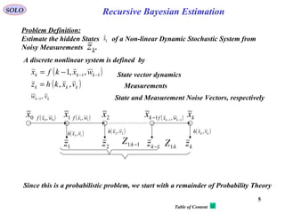
Recursive Bayesian EstimationSOLO
( ) ( ) ( )
( ) ( )kvkkk
xkkwkkkk
vpgivenvxhz
xpuwpgivenwuxfx
:
,,:, 011111 0
+=
+= −−−−−
kx1−kx
kz1−kz
( ) 111, −−− + kkk wuxf
( ) kk vxh +
Markov Processes
( ) ( )[ ]111 ,| −−− −= kkkwkk uxfxpxxptherefore
( ) ( )[ ]kkvkk xhzpxzp −=|and
For additive noise
we have
( )
( )kkk
kkkk
xhzv
uxfxw
−=
−= −−− 111 ,
Analytic Computations of and (continue – 1)( )kk xzp |( )1| −kk xxp](https://image.slidesharecdn.com/3-recursivebayesianestimation-150113075152-conversion-gate02/85/3-recursive-bayesian-estimation-77-320.jpg)

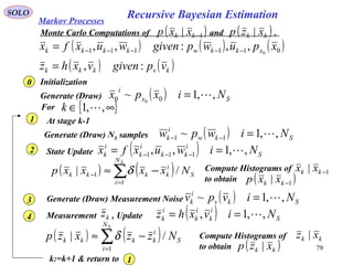
![SOLO
Stochastic Processes deal with systems corrupted by noise. A description of those processes is
given in “Stochastic Processes” Presentation. Here we give only one aspect of those processes.
( ) ( ) ( ) [ ]fttttwddttxftxd ,, 0∈+=
A continuous dynamic system is described by:
Stochastic Processes
( )tx - n- dimensional state vector
( )twd - n- dimensional process noise vector
Assuming system measurements at discrete time tk given by:
( ) ( )( ) [ ]fkkkkk tttvttxhtz ,,, 0∈=
kv - m- dimensional measurement noise vector at tk
We are interested in the probability of the state at time t given the set of discrete
measurements until (included) time tk < t.
x
( )kZtxp |,
{ }kk zzzZ ,,, 21 = - set of all measurements up to and including time tk.
The time evolution of the probability density function is described by the
Fokker–Planck equation.](https://image.slidesharecdn.com/3-recursivebayesianestimation-150113075152-conversion-gate02/85/3-recursive-bayesian-estimation-80-320.jpg)
![A solution to the one-dimensional
Fokker–Planck equation, with both the
drift and the diffusion term. The initial
condition is a Dirac delta function in
x = 1, and the distribution drifts
towards x = 0.
The Fokker–Planck equation describes the time evolution of
the probability density function of the position of a particle, and
can be generalized to other observables as well. It is named after
Adriaan Fokker and Max Planck and is also known as the
Kolmogorov forward equation. The first use of the Fokker–
Planck equation was the statistical description of Brownian
motion of a particle in a fluid.
In one spatial dimension x, the Fokker–Planck equation for a
process with drift D1(x,t) and diffusion D2(x,t) is
More generally, the time-dependent probability distribution
may depend on a set of N macrovariables xi. The general
form of the Fokker–Planck equation is then
where D1
is the drift vector and D2
the diffusion tensor; the latter results from the presence of the
stochastic force.
Fokker – Planck Equation
Adriaan Fokker
1887 - 1972
Max Planck
1858 - 1947
SOLO
Adriaan Fokker
„Die mittlere Energie rotierender
elektrischer Dipole im Strahlungsfeld"
Annalen der Physik 43, (1914) 810-
820
Max Plank, „Ueber einen Satz der
statistichen Dynamik und eine
Erweiterung in der Quantumtheorie“,
Sitzungberichte der Preussischen
Akadademie der Wissenschaften
(1917) p. 324-341
Stochastic Processes
( ) ( ) ( )[ ] ( ) ( )[ ]txftxD
x
txftxD
x
txf
t
,,,,, 22
2
1
∂
∂
+
∂
∂
−=
∂
∂
( )[ ] ( )[ ]∑∑∑ = == ∂∂
∂
+
∂
∂
−=
∂
∂ N
i
N
j
Nji
ji
N
i
Ni
i
ftxxD
xx
ftxxD
x
f
t 1 1
1
2
2
1
1
1
,,,,,, ](https://image.slidesharecdn.com/3-recursivebayesianestimation-150113075152-conversion-gate02/85/3-recursive-bayesian-estimation-81-320.jpg)
![Fokker – Planck Equation (continue – 1)
The Fokker–Planck equation can be used for computing the probability densities of stochastic
differential equations.
where is the state and is a standard M-dimensional Wiener process. If the initial
probability distribution is , then the probability distribution of the state
is given by the Fokker – Planck Equation with the drift and diffusion terms:
Similarly, a Fokker–Planck equation can be derived for Stratonovich stochastic differential
equations. In this case, noise-induced drift terms appear if the noise strength is state-dependent.
SOLO
Consider the Itô stochastic differential equation:
( ) ( ) ( )[ ] ( ) ( )[ ]txftxD
x
txftxD
x
txf
t
,,,,, 22
2
1
∂
∂
+
∂
∂
−=
∂
∂](https://image.slidesharecdn.com/3-recursivebayesianestimation-150113075152-conversion-gate02/85/3-recursive-bayesian-estimation-82-320.jpg)
![Fokker – Planck Equation (continue – 2)
Derivation of the Fokker–Planck Equation
SOLO
Start with ( ) ( ) ( )11|1, 111
|, −−− −−−
= kxkkxxkkxx xpxxpxxp kkkkk
and ( ) ( ) ( ) ( )∫∫
+∞
∞−
−−−
+∞
∞−
−− −−−
== 111|11, 111
|, kkxkkxxkkkxxkx xdxpxxpxdxxpxp kkkkkk
define ( ) ( )ttxxtxxttttt kkkk ∆−==∆−== −− 11 ,,,
( ) ( )[ ] ( ) ( ) ( ) ( )[ ] ( ) ( )[ ] ( )∫
+∞
∞−
∆−∆− ∆−∆−∆−= ttxdttxpttxtxptxp ttxttxtxtx ||
Let use the Characteristic Function of
( ) ( ) ( ) ( ) ( )[ ]{ } ( ) ( ) ( ) ( )[ ] ( ) ( ) ( ) ( )ttxtxtxtxdttxtxpttxtxss ttxtxttxtx ∆−−=∆∆−∆−−−=Φ ∫
+∞
∞−
∆−∆−∆ |exp: ||
( ) ( ) ( ) ( )[ ]ttxtxp ttxtx ∆−∆− ||
The inverse transform is ( ) ( ) ( ) ( )[ ] ( ) ( )[ ]{ } ( ) ( ) ( )∫
∞+
∞−
∆−∆∆− Φ∆−−=∆−
j
j
ttxtxttxtx sdsttxtxs
j
ttxtxp || exp
2
1
|
π
Using Chapman-Kolmogorov Equation we obtain:
( ) ( )[ ] ( ) ( )[ ]{ } ( ) ( ) ( )
( ) ( ) ( ) ( )[ ]
( ) ( )[ ] ( )
( ) ( )[ ]{ } ( ) ( ) ( ) ( ) ( )[ ] ( )ttxdsdttxpsttxtxs
j
ttxdttxpsdsttxtxs
j
txp
j
j
ttxttxtx
ttx
ttxtxp
j
j
ttxtxtx
ttxtx
∆−∆−Φ∆−−=
∆−∆−Φ∆−−=
∫ ∫
∫ ∫
∞+
∞−
∞+
∞−
∆−∆−∆
+∞
∞−
∆−
∆−
∞+
∞−
∆−∆
∆−
|
|
|
exp
2
1
exp
2
1
|
π
π
Stochastic Processes](https://image.slidesharecdn.com/3-recursivebayesianestimation-150113075152-conversion-gate02/85/3-recursive-bayesian-estimation-83-320.jpg)
![Fokker – Planck Equation (continue – 3)
Derivation of the Fokker–Planck Equation (continue – 1)
SOLO
The Characteristic Function can be expressed in terms of the moments about x (t-Δt) as:
( ) ( )[ ] ( ) ( )[ ]{ } ( ) ( ) ( ) ( ) ( )[ ] ( )ttxdsdttxpsttxtxs
j
txp
j
j
ttxttxtxtx ∆−∆−Φ∆−−= ∫ ∫
+∞
∞−
∞+
∞−
∆−∆−∆ |exp
2
1
π
( ) ( ) ( ) ( )
( ) ( ) ( ) ( )[ ] ( ){ }∑
∞
=
∆−∆∆−∆ ∆−∆−−
−
+=Φ
1
|| |
!
1
i
i
ttxtx
i
ttxtx ttxttxtxE
i
s
s
Therefore
( ) ( )[ ] ( ) ( )[ ]{ } ( )
( ) ( ) ( ) ( )[ ] ( ){ } ( ) ( )[ ] ( )ttxdsdttxpttxttxtxE
i
s
ttxtxs
j
txp
j
j
ttx
i
i
ttxtx
i
tx ∆−∆−
∆−∆−−
−
+∆−−= ∫ ∫ ∑
+∞
∞−
∞+
∞−
∆−
∞
=
∆−
1
| |
!
1exp
2
1
π
Use the fact that ( ) ( ) ( )[ ]{ } ( ) ( ) ( )[ ]
( )[ ]
,2,1,01exp
2
1
=
∂
∆−−∂
−=∆−−−∫
∞+
∞−
i
tx
ttxtx
sdttxtxss
j i
i
i
j
j
i δ
π
( ) ( )[ ] ( ) ( )[ ]{ } ( ) ( )[ ] ( )
( ) ( ) ( )[ ]
( )[ ]
( ) ( )[ ] ( ){ } ( ) ( )[ ] ( )∫∑
∫ ∫
∞+
∞−
∞
=
∆−
+∞
∞−
∆−
∞+
∞−
∆−∆−∆−∆−−
∂
∆−−∂−
+
∆−∆−∆−−=
1
|
!
1
exp
2
1
i
ttx
i
i
ii
ttx
j
j
tx
ttxdttxpttxttxtxE
tx
ttxtx
i
ttxdttxpsdttxtxs
j
txp
δ
π
where δ [u] is the Dirac delta function:
[ ] { } ( ) [ ] ( ) ( ) ( ) ( ) ( )000..0exp
2
1
FFFtsuFFduuuFsdus
j
u
j
j
==∀== −+
+∞
∞−
∞+
∞−
∫∫ δ
π
δ
Stochastic Processes](https://image.slidesharecdn.com/3-recursivebayesianestimation-150113075152-conversion-gate02/85/3-recursive-bayesian-estimation-84-320.jpg)
![Fokker – Planck Equation (continue – 4)
Derivation of the Fokker–Planck Equation (continue – 2)
SOLO
[ ] ( ){ } ( ) [ ] ( ) ( ) ( ) ( ) ( )afafaftsufufduuaufsduas
j
ua au
j
j
==∀=−−=− −+=
+∞
∞−
∞+
∞−
∫∫ ..exp
2
1
δ
π
δ
[ ] ( ){ } ( ) ( ) { } ( ) ( ) { }∫∫∫
∞+
∞−
∞+
∞−
∞+
∞−
=→=−
−
=−
j
j
j
j
j
j
sdussFs
j
uf
du
d
sdussF
j
ufsduass
j
ua
ud
d
exp
2
1
exp
2
1
exp
2
1
πππ
δ
( ) [ ] ( ) ( ){ } ( ) ( ){ }
{ } ( ) { } { } ( ) ( )
au
j
j
j
j
j
j
j
j
ud
ufd
sdsFass
j
sdduusufass
j
sdduuasufs
j
dusduass
j
ufduua
ud
d
uf
=
∞+
∞−
∞+
∞−
∞+
∞−
∞+
∞−
+∞
∞−
+∞
∞−
∞+
∞−
+∞
∞−
−=
−
=−
−
=
−
−
=−
−
=−
∫∫ ∫
∫ ∫∫ ∫∫
exp
2
1
expexp
2
1
exp
2
1
exp
2
1
ππ
ππ
δ
[ ] ( ) ( ){ } ( ) ( ) { } ( ) ( ) { }∫∫∫
∞+
∞−
∞+
∞−
∞+
∞−
=→=−
−
=−
j
j
i
i
ij
j
j
j
i
i
i
i
sdussFs
j
uf
du
d
sdussF
j
ufsduass
j
ua
ud
d
exp
2
1
exp
2
1
exp
2
1
πππ
δ
( ) [ ] ( ) ( ) ( ){ } ( ) ( ) ( ){ }
( ) { } ( ) { } ( ) ( ) { } ( ) ( )
au
i
i
i
j
j
i
ij
j
i
i
j
j
i
ij
j
i
i
i
i
ud
ufd
sdassFs
j
sdduusufass
j
sdduuasufs
j
dusduass
j
ufduua
ud
d
uf
=
−=
−
=−
−
=
−
−
=−
−
=−
∫∫ ∫
∫ ∫∫ ∫∫
∞+
∞−
∞+
∞−
∞+
∞−
∞+
∞−
+∞
∞−
+∞
∞−
∞+
∞−
+∞
∞−
1exp
2
1
expexp
2
1
exp
2
1
exp
2
1
ππ
ππ
δ
Useful results related to integrals involving Delta (Dirac) function
Stochastic Processes](https://image.slidesharecdn.com/3-recursivebayesianestimation-150113075152-conversion-gate02/85/3-recursive-bayesian-estimation-85-320.jpg)
![Fokker – Planck Equation (continue – 5)
Derivation of the Fokker–Planck Equation (continue – 3)
SOLO
( ) ( )[ ]{ }
( ) ( )[ ]
( ) ( )[ ] ( ) ( ) ( )[ ] ( ) ( )[ ] ( ) ( ) ( )[ ]txpttxdttxpttxtxttxdttxpsdttxtxs
j
ttxttxttx
ttxtx
j
j
∆−
+∞
∞−
∆−
+∞
∞−
∆−
∆−−
∞+
∞−
=∆−∆−∆−−=∆−∆−∆−− ∫∫ ∫ δ
π
δ
exp
2
1
( ) ( ) ( )[ ]
( )[ ] ( ) ( ) ( ) ( )[ ] ( ){ } ( ) ( )[ ] ( )
( ) ( ) ( )[ ]
( )[ ] ( ) ( ) ( ) ( )[ ] ( ){ } ( ) ( )[ ] ( )
( ) ( ) ( ) ( ) ( )[ ] ( ){ } ( ) ( )[ ]( )
( )[ ]∑
∑ ∫
∫∑
∞
=
=∆
∆−∆−
∞
=
∞+
∞−
∆−∆−
+∞
∞−
∞
=
∆−∆−
∂
∆−∆−−∂−
=
∆−∆−∆−∆−−
∂
∆−−∂−
=
∆−∆−∆−∆−−
∂
∆−−∂−
1
0
|
1
|
1
|
|
!
1
|
!
1
|
!
1
i
t
i
ttx
i
ttxtx
ii
i
ttx
i
ttxtxi
ii
i
ttx
i
ttxtxi
ii
tx
txpttxttxtxE
i
ttxdttxpttxttxtxE
tx
ttxtx
i
ttxdttxpttxttxtxE
tx
ttxtx
i
δ
δ
( ) [ ] ( ) ( ) ( )
[ ]
[ ] ( )
auau
i
i
i
i
i
i
i
i
i
ud
ufd
duua
uad
d
uf
ud
ufd
duua
ud
d
uf
==
=−
−
→−=− ∫∫
+∞
∞−
+∞
∞−
δδ 1We found
( ) ( )[ ] ( ) ( )[ ] ( ) ( ) ( ) ( ) ( )[ ] ( ){ } ( ) ( )[ ]( )
( )[ ]∑
∞
=
=∆
∆−∆−
∆−
∂
∆−∆−−∂−
+=
1
0
| |
!
1
i
t
i
ttx
i
ttxtx
ii
ttxtx
tx
txpttxttxtxE
i
txptxp
( ) ( )[ ] ( ) ( )[ ] ( ) ( ) ( )[ ] ( ){ } ( ) ( )[ ]( )
( )[ ]∑
∞
=
∆−
→∆
∆−
→∆ ∂
∆−∆−−∂
∆
−
=
∆
−
1
00
|1
lim
!
1
lim
i
i
ttx
ii
t
i
ttxtx
t tx
txpttxttxtxE
tit
txptxp
Therefore
Rearranging, dividing by Δt, and tacking the limit Δt→0, we obtain:
Stochastic Processes](https://image.slidesharecdn.com/3-recursivebayesianestimation-150113075152-conversion-gate02/85/3-recursive-bayesian-estimation-86-320.jpg)
![Fokker – Planck Equation (continue – 6)
Derivation of the Fokker–Planck Equation (continue – 4)
SOLO
We found ( ) ( )[ ] ( ) ( )[ ] ( ) ( ) ( ) ( ) ( )[ ] ( ){ } ( ) ( )[ ]( )
( )[ ]∑
∞
=
∆−∆−
→∆
∆−
→∆ ∂
∆−∆−−∂
∆
−
=
∆
−
1
|
00
|1
lim
!
1
lim
i
i
ttx
i
ttxtx
i
t
i
ttxtx
t tx
txpttxttxtxE
tit
txptxp
Define: ( ) ( )[ ] ( ) ( ) ( ) ( )[ ] ( ){ }
t
ttxttxtxE
txtxm
i
ttxtx
t
i
∆
∆−∆−−
=−
∆−
→∆
−
|
lim:
|
0
Therefore ( ) ( )[ ] ( ) ( ) ( )[ ] ( ) ( )[ ]( )
( )[ ]∑
∞
=
−
∂
−∂−
=
∂
∂
1 !
1
i
i
tx
iii
tx
tx
txptxtxm
it
txp
( ) ( )ttxtx
t
∆−=
→∆
−
0
lim: and:
This equation is called the Stochastic Equation or Kinetic Equation.
It is a partial differential equation that we must solve, with the initial condition:
( ) ( )[ ] ( )[ ]000 0 txptxp tx ===
Stochastic Processes](https://image.slidesharecdn.com/3-recursivebayesianestimation-150113075152-conversion-gate02/85/3-recursive-bayesian-estimation-87-320.jpg)
![Fokker – Planck Equation (continue – 7)
Derivation of the Fokker–Planck Equation (continue – 5)
SOLO
We want to find px(t) [x(t)] where x(t) is the solution of
( ) ( ) ( ) [ ]fg ttttntxf
dt
txd
,, 0∈+=
( ){ } 0: == tnEn gg
( )tng
( ) ( )[ ] ( ) ( )[ ]{ } ( ) ( )τδττ −=−− ttQnntntnE gggg
ˆˆ
Wiener (Gauss) Process
( ) ( )[ ] ( ) ( )[ ] ( ){ } [ ] ( ){ } [ ]{ } ( )tQnEtxnE
t
ttxttxtxE
txtxm gg
t
===
∆
∆−∆−−
=−
→∆
−
22
2
2
0
2
|
|
lim:
( ) ( )[ ] ( ) ( )[ ] ( ){ } ( ) ( ) ( ) ( ) ( )txfnEtxftx
td
txd
E
t
ttxttxtxE
txtxm g
t
,,|
|
lim:
0
0
1
=+=
=
∆
∆−∆−−
=−
→∆
−
( ) ( )[ ] ( ) ( )[ ] ( ){ } 20
|
lim:
0
>=
∆
∆−∆−−
=−
→∆
− i
t
ttxttxtxE
txtxm
i
t
i
Therefore we obtain:
( ) ( )[ ] ( )[ ] ( ) ( )[ ]( )
( )
( ) ( ) ( )[ ]
( )[ ]2
2
2
1,
tx
txp
tQ
tx
txpttxf
t
txp txtxtx
∂
∂
+
∂
∂
−=
∂
∂
Stochastic Processes
Fokker–Planck Equation
Return to Daum](https://image.slidesharecdn.com/3-recursivebayesianestimation-150113075152-conversion-gate02/85/3-recursive-bayesian-estimation-88-320.jpg)


![99
Recursive Bayesian EstimationSOLO
Linear Gaussian Markov Systems (continue – 3)
111111 −−−−−− Γ++Φ= kkkkkkk wuGxx
Prediction phase (before zk measurement)
{ } { } { }
0
1:111111:1111:11| |||:ˆ −−−−−−−−−− Γ++Φ== kkkkkkkkkkkk ZwEuGZxEZxEx
or 111|111|
ˆˆ −−−−−− +Φ= kkkkkkk uGxx
The expectation is
{ }[ ] { }[ ]{ }
( )[ ] ( )[ ]{ }1:1111|111111|111
1:11|1|1|
|ˆˆ
|ˆˆ:
−−−−−−−−−−−−−
−−−−
Γ+−ΦΓ+−Φ=
−−=
k
T
kkkkkkkkkkkk
k
T
kkkkkkkk
ZwxxwxxE
ZxExxExEP
( ) ( ){ } ( ){ }
( ){ } { } T
k
Q
T
kkk
T
k
T
kkkkk
T
k
T
kkkkk
T
k
P
T
kkkkkkk
wwExxwE
wxxExxxxE
kk
11111
0
1|1111
1
0
11|11111|111|111
ˆ
ˆˆˆ
1|1
−−−−−−−−−−
−−−−−−−−−−−−−−
ΓΓ+Φ−Γ+
Γ−Φ+Φ−−Φ=
−−
T
kk
T
kkkkkk QPP 1111|111| −−−−−−− ΓΓ+ΦΦ=
{ } ( )1|1|1:1 ,ˆ;| −−− = kkkkkkk PxxZxP N
Since is a Linear Combination of Independent
Gaussian Random Variables:
111111 −−−−−− Γ++Φ= kkkkkkk wuGxx](https://image.slidesharecdn.com/3-recursivebayesianestimation-150113075152-conversion-gate02/85/3-recursive-bayesian-estimation-99-320.jpg)

![101
( ) ( )kkkv Rvvp ,0;N=
kkkk vxHz +=
Consider a Gaussian vector , where ,
measurement, , where the Gaussian noise
is independent of and .
v
kx ( ) [ ]1|1| ,; −−= kkkkkkx Pxxxp
N
kx
( ) ( ) ( ) ( )∫∫
+∞
∞−
+∞
∞−
== kkxkkxzkkkzxkz xdxpxzpxdzxpzp |, |,
is Gaussian with( )kz zp ( ) ( ) ( ) ( ) 1|
0
−=+=+= kkkkkkkkk xHvExEHvxHEzE
( ) ( )[ ] ( )[ ]{ } [ ][ ]{ }
( )[ ] ( )[ ]{ } [ ]{ }
[ ]{ } [ ]{ } { } k
T
kkkk
T
kk
T
k
T
kkkk
T
kkkkk
T
k
T
kkkkkkk
T
kkkkkkkkkk
T
kkkkkkkkkkkk
T
kkkkk
RHPHvvEHxxvEvxxEH
HxxxxEHvxxHvxxHE
xHvxHxHvxHEzEzzEzEz
+=+−−−−
−−=+−+−=
−+−+=−−=
−−−
−−−−
−−
1|
0
1|
0
1|
1|1|1|1|
1|1|cov
( )
( ) ( )
( )[ ] ( )[ ] ( )[ ]
−−+−−−−
+−
=
−
xHzRHPHxHz
RHPH
zp TT
Tpz
ˆˆ
2
1
exp
2
1 1
2/12/
π
( )
( )
( ) ( )
−−−= −
−
−−
−
−− 1|
1
1|1|2/1
1|
2/1:1|
2
1
exp
2
1
|1:1 kkkkk
T
kkk
kk
nkkZx xxPxx
P
Zxp kk
π
( ) ( )
( )
( ) ( )
−−−=−= −
kkk
T
kkkpkkkvkkxz xHzRxHz
R
xHzpxzp 1
2/12/|
2
1
exp
2
1
|
π
Recursive Bayesian EstimationSOLO
Linear Gaussian Markov Systems (continue – 5)
Correction Step (after zk measurement) 1st
Way (continue – 1)](https://image.slidesharecdn.com/3-recursivebayesianestimation-150113075152-conversion-gate02/85/3-recursive-bayesian-estimation-101-320.jpg)
![102
Recursive Bayesian EstimationSOLO
Linear Gaussian Markov Systems (continue – 6)
kkkk vxHz +=
( ) ( )Rvvpv ,0;N=
( )
( )
−= −
vRv
R
vp T
pv
1
2/12/
2
1
exp
2
1
π
Correction Step (after zk measurement) 1st
Way (continue – 2)
( )
( )
( ) ( )
−−−= −
−
−−
−
−− 1|
1
1|1|2/1
1|
2/1:1|
2
1
exp
2
1
|1:1 kkkkk
T
kkk
kk
nkkZx xxPxx
P
Zxp kk
π
( ) ( )
( )
( ) ( )
−−−=−= −
kkk
T
kkkpkkkvkkxz xHzRxHz
R
xHzpxzp 1
2/12/|
2
1
exp
2
1
|
π
( )
( )
[ ] [ ] [ ]
−+−−
+
= −
−
−−
−
1|
1
1|1|2/1
1|
2/
ˆˆ
2
1
exp
2
1
kkkk
T
kkkk
T
kkk
k
T
kkkk
p
kz xHzRHPHxHz
RHPH
zp
π
( ) ( ) ( )
( )
( )
( ) ( ) ( ) ( ) [ ] [ ] [ ]
−+−+−−−−−−⋅
+
==
−
−
−−−
−
−−
−
−
−−
−
1|
1
1|1|1|
1
1|1|
1
2/1
1|
2/12/1
1|2/1:1
1:1
:1
ˆˆ
2
1
2
1
2
1
exp
2
1
|
||
|
kkkkk
T
kkkk
T
kkkkkkkkk
T
kkkkkkk
T
kkk
k
T
kkkk
kkknkk
kkkk
kk
xHzRHPHxHzxxPxxxHzRxHz
RHPH
RPZzp
Zxpxzp
Zxp
π
from which](https://image.slidesharecdn.com/3-recursivebayesianestimation-150113075152-conversion-gate02/85/3-recursive-bayesian-estimation-102-320.jpg)
![103
( ) ( ) ( ) ( ) ( ) [ ] ( )1|
1
1|1|1|
1
1|1|
1
−
−
−−−
−
−−
−
−+−−−−+−− kkkk
T
kkkkk
T
kkkkkkkkk
T
kkkkkkk
T
kkk xHzHPHRxHzxxPxxxHzRxHz
( )[ ] ( )[ ] ( ) ( )
( ) [ ] ( ) ( ) [ ]{ }( )
( ) ( ) ( ) ( ) ( ) [ ]( )1|
11
1|1|1|
1
1|1|
1
1|
1|
1
1|
1
1|1|
1
1|1|
1|
1
1|1|1|1|
1
1|1|
−
−−
−−−
−
−−
−
−
−
−
−
−
−−
−
−−
−
−
−−−−
−
−−
−+−+−−−−−−
−+−−=−+−−
−−+−−−−−−=
kkkkk
T
kkk
T
kkkkkkkk
T
kkkkkkkkk
T
k
T
kkk
kkkk
T
kkkkkk
T
kkkkkkkk
T
kkkkk
T
kkkk
kkkkk
T
kkkkkkkkkkkk
T
kkkkkkkk
xxHRHPxxxxHRxHzxHzRHxx
xHzHPHRRxHzxHzHPHRxHz
xxPxxxxHxHzRxxHxHz
[ ] [ ] 1111
1|
1111
1|
1 −−−−
−
−−−−
−
−
++/−/=+− k
T
kkk
T
kkkkkkk
LemmaMatrixInverse
T
kkkkkk RHHRHPHRRRHPHRRwe have
Define:
[ ] [ ] 1
1|
1
1|
1
1|
1
1|
111
1|| :
−
−
−
−
−
−
−
−
−−−
− +−=+= kk
T
k
T
kkkkkkkkkk
LemmaMatrixInverse
kk
T
kkkkk PHHPHRHPPHRHPP
( )[ ] ( )[ ]1|
1
|1|
1
|1|
1
|1| −
−
−
−
−
−
− −+−−+−= kkkkk
T
kkkkkkkk
T
kkkkk
T
kkkkkk xHzRHPxxPxHzRHPxx
( )
( )
( )[ ] ( )[ ]
−+−−+−−⋅= −
−
−
−
−
−
− 1|
1
|1|
1
|1|
1
|1|2/1
|
2/:1|
2
1
exp
2
1
| kkkkk
T
kkkkkkkk
T
kkkkk
T
kkkkkk
kk
nkkzx xHzRHPxxPxHzRHPxx
P
Zxp
π
Recursive Bayesian EstimationSOLO
Linear Gaussian Markov Systems (continue – 7)
Correction Step (after zk measurement) 1st
Way (continue – 3)
then ( ) ( ) ( ) ( ) ( ) [ ] ( )1|
1
1|1|1|
1
1|1|
1
−
−
−−−
−
−−
−
−+−−−−+−− kkkkk
T
kkkk
T
kkkkkkkkk
T
kkkkkkk
T
kkk xHzRHPHxHzxxPxxxHzRxHz
( ) ( ) ( ) ( ) ( ) ( )
( ) ( )( ) ( ) ( )1|
1
|1|1|
1
||
1
1|
1|
1
|
1
|1|1|
1
|
1
||
1
1|
−
−
−−
−−
−
−
−−
−−
−−−
−
−−+−−−
−−−−−=
kkkkk
T
kkkkkkkkkkkk
T
kkkk
kkkkk
T
kkkkk
T
kkkkkkkk
T
kkkkkkkkk
T
kkkk
xxPxxxxPPHRxHz
xHzRHPPxxxHzRHPPPHRxHz
](https://image.slidesharecdn.com/3-recursivebayesianestimation-150113075152-conversion-gate02/85/3-recursive-bayesian-estimation-103-320.jpg)
![104
then
( )kkzx
x
Zxp
k
:1| |max
( )
{ }kk
kkkkk
T
kkkkkkkk
ZxE
xHzRHPxxx
:1
1|
1
|1|
*
|
|
ˆˆ:ˆ
=
−+== −
−
−
Recursive Bayesian EstimationSOLO
Linear Gaussian Markov Systems (continue – 8)
Correction Step (after zk measurement) 1st
Way (continue – 4)
( )
( )
( )[ ] ( )[ ]
−+−−+−−⋅= −
−
−
−
−
−
− 1|
1
1|
1
|1|
1
1|2/1
|
2/:1|
2
1
exp
2
1
| kkkkk
T
kkkkkk
T
kkkkk
T
kkkk
kk
nkkzx xHzRHxxPxHzRHxx
P
Zxp
π
where:[ ] ( )( ){ }k
T
kkkkkkkk
T
kkkkk ZxxxxEHRHPP :1||
111
1||
ˆˆ: −−=+=
−−−
−](https://image.slidesharecdn.com/3-recursivebayesianestimation-150113075152-conversion-gate02/85/3-recursive-bayesian-estimation-104-320.jpg)
![105
{ } ( ) ( )
ki
kkkkkkkkkkkkkkkkk zzKxxHzKxZxEx 1|1|1|1|:1| ˆ| −−−− −+=−+==
Recursive Bayesian EstimationSOLO
Linear Gaussian Markov Systems (continue – 9)
Summary 1st
Way – Kalman Filter
Initial Conditions:
[ ] 111
1|| :
−−−
− += kk
T
kkkkk HRHPP
Prediction phase (before zk measurement)
111|111|
ˆˆ −−−−−− +Φ= kkkkkkk uGxx
Correction Step (after zk measurement)
T
kk
T
kkkkkk QPP 1111|111| −−−−−−− ΓΓ+ΦΦ=
1
|:
−
= k
T
kkkk RHPK
{ }00|0
ˆ xEx = ( ) ( ){ }T
xxxxEP 0|000|000|0
ˆˆ: −−=
kkkk wxHz += { } { } { }
0
1:11|1:11:11| |ˆ||ˆ −−−−− +=+== kkkkkkkkkkkkk ZwExHZwxHEZzEz
1|1|
ˆˆ −− = kkkkk xHz](https://image.slidesharecdn.com/3-recursivebayesianestimation-150113075152-conversion-gate02/85/3-recursive-bayesian-estimation-105-320.jpg)
![106
Recursive Bayesian EstimationSOLO
Linear Gaussian Markov Systems (continue – 10)
kkkk vxHz +=
( ) ( )Rvvpv ,0;N= ( )
( )
−= −
vRv
R
vp T
pv
1
2/12/
2
1
exp
2
1
π
( )
( )
[ ] [ ] [ ]
−+−−
+
= −
−
−−
−
1|
1
1|1|2/1
1|
2/
ˆˆ
2
1
exp
2
1
kkkkk
T
kkkk
T
kkkk
k
T
kkkk
p
kz xHzRHPHxHz
RHPH
zp
π
from which { } 1|1:11|
ˆ|ˆ −−− == kkkkkkk xHZzEz
( ) ( ){ } kk
T
kkkkk
T
kkkkkk
zz
kk SRHPHZzzzzEP =+=−−= −−−−− :ˆˆ 1|1:11|1|1|
[ ][ ]{ }
[ ] ( )[ ]{ } T
kkkk
T
kkkkkkkk
k
T
kkkkkk
xz
kk
HPZvxxHxxE
ZzzxxEP
1|1:11|1|
1:11|1|1|
ˆˆ
ˆˆ
−−−−
−−−−
=+−−=
−−=
We also have
Correction Step (after zk measurement) 2nd
Way
Define the innovation: 1|1|
ˆˆ: −− −=−= kkkkkk xHzzzi](https://image.slidesharecdn.com/3-recursivebayesianestimation-150113075152-conversion-gate02/85/3-recursive-bayesian-estimation-106-320.jpg)
![107
Recursive Bayesian EstimationSOLO
Joint and Conditional Gaussian Random Variables
=
k
k
k
z
x
yDefine: assumed that they are Gaussian distributed
Prediction phase (before zk measurement) 2nd
way (continue -1)
{ }
=
=
−
−
−
−
−
1|
1|
1:1
1:1
1:1
ˆ
ˆ
|
|
|
kk
kk
kk
kk
kk
z
x
Zz
Zx
EZyE
=
−
−
−
−
=
−−
−−
−
−
−
−
−
− zz
kk
zx
kk
xz
kk
xx
kk
k
T
kkk
kkk
kkk
kkkyy
kk
PP
PP
Z
zz
xx
zz
xx
EP
1|1|
1|1|
1:1
1|
1|
1|
1|
1|
ˆ
ˆ
ˆ
ˆ
where: [ ][ ]{ } 1|1:11|1|1|
ˆˆ −−−−− =−−= kkk
T
kkkkkk
xx
kk PZxxxxEP
[ ][ ]{ } kk
T
kkkkk
T
kkkkkk
zz
kk SRHPHZzzzzEP =+=−−= −−−−− :ˆˆ 1|1:11|1|1|
[ ][ ]{ } T
kkkk
T
kkkkkk
xz
kk HPZzzxxEP 1|1:11|1|1| ˆˆ −−−−− =−−=
Linear Gaussian Markov Systems (continue – 11)](https://image.slidesharecdn.com/3-recursivebayesianestimation-150113075152-conversion-gate02/85/3-recursive-bayesian-estimation-107-320.jpg)


![111
Recursive Bayesian EstimationSOLO
Joint and Conditional Gaussian Random Variables
Prediction phase (before zk measurement) 2nd
way (continue – 5)
=
−−
−−
−
−−
−−
zz
kk
zx
kk
xz
kk
xx
kk
zz
kk
zx
kk
xz
kk
xx
kk
TT
TT
PP
PP
1|1|
1|1|
1
1|1|
1|1|
1
1|1|1|
1
1|
1|
1
1|1|1|
1
1|
1|
1
1|1|1|
1
1|
−
−−−
−
−
−
−
−−−
−
−
−
−
−−−
−
−
−=
−=
−=
zz
kk
xz
kk
xz
kk
xx
kk
xz
kk
xx
kk
zx
kk
zz
kk
zz
kk
kkzxkkzzkkxzkkxxkkxx
PPTT
TTTTP
PPPPT
( ) ( )k
xz
kk
xx
kkk
xx
kk
T
k
xz
kk
xx
kkk TTTTTq ςξςξ 1|
1
1|1|1|
1
1| −
−
−−−
−
− ++=
1|1| ˆ:&ˆ: −− −=−= kkkkkkkk zzxx ςξ
( )
( )[ ] ( )[ ]
−−−−−−−=
−=
−−−−−
−
−
−
−
1|1|1|1|1|2/1
1|
2/1
1|
2/1
1|
2/1
1|
|
ˆˆˆˆ
2
1
exp
2
2
2
1
exp
2
2
|
kkkkkkk
xx
kk
T
kkkkkkk
yy
kk
zz
kk
yy
kk
zz
kk
kkzx
zzKxxTzzKxx
P
P
q
P
P
zxp
π
π
π
π
( )1|
1
1|1|1|
1
1|1| ˆˆ −
−
−−−
−
−− −−−=+ kkk
K
zz
kk
xz
kkkkkk
xx
kk
xz
kkk zzPPxxTT
k
ςξ
Linear Gaussian Markov Systems (continue – 15)](https://image.slidesharecdn.com/3-recursivebayesianestimation-150113075152-conversion-gate02/85/3-recursive-bayesian-estimation-111-320.jpg)
![112
Recursive Bayesian EstimationSOLO
Joint and Conditional Gaussian Random Variables
Prediction phase (before zk measurement) 2nd
Way (continue – 6)
( ) ( )[ ] ( )[ ]
−−−−−−−= −
−
−−−−−
−
−−− 1|
1
1|1|1|1|1|
1
1|1|1|| ˆˆˆˆ
2
1
exp| kkk
xx
kk
xz
kkkkk
xx
kk
T
kkk
xx
kk
xz
kkkkkkkzx zzPPxxTzzPPxxczxp
From this we can see that
{ } ( )1|
1
1|1|1|| ˆˆˆ| −
−
−−− −+== kkk
K
zz
kk
xz
kkkkkkkk zzPPxxzxE
k
( )( ){ }
T
k
zz
kkk
xx
kk
zx
kk
zz
kk
xz
kk
xx
kk
xx
kkk
T
kkkkkk
xx
kk
KPKP
PPPPTZxxxxEP
1|1|
1|
1
1|1|1|
1
1|:1|||
ˆˆ
−−
−
−
−−−
−
−
−=
−==−−=
[ ][ ]{ } 1|1:11|1|1|
ˆˆ −−−−− =−−= kkk
T
kkkkkk
xx
kk PZxxxxEP
[ ][ ]{ } k
T
kkkkkk
T
kkkkkk
zz
kk SHPHRZzzzzEP =+=−−= −−−−− :ˆˆ 1|1:11|1|1|
[ ][ ]{ } T
kkkk
T
kkkkkk
xz
kk HPZzzxxEP 1|1:11|1|1| ˆˆ −−−−− =−−=
Linear Gaussian Markov Systems (continue – 16)](https://image.slidesharecdn.com/3-recursivebayesianestimation-150113075152-conversion-gate02/85/3-recursive-bayesian-estimation-112-320.jpg)
![113
Recursive Bayesian EstimationSOLO
Joint and Conditional Gaussian Random Variables
Prediction phase (before zk measurement) 2nd
Way (continue – 7)
From this we can see that
( ) [ ] 111
1|1|
1
1|1|1||
−−−
−−
−
−−− +=+−= kk
T
kkkkkk
T
kkkkk
T
kkkkkkk HRHPPHHPHRHPPP
( ) 1
1|
1
1|1|
1
1|1|
−
−
−
−−
−
−− =+== k
T
kkk
T
kkkkk
T
kkk
zz
kk
xz
kkk SHPHPHRHPPPK
Linear Gaussian Markov Systems (continue – 17)
kk
T
kkkkk KSKPP −= −1||
or
[ ][ ]{ } 1|1:11|1|1|
ˆˆ −−−−− =−−= kkk
T
kkkkkk
xx
kk PZxxxxEP
[ ][ ]{ } k
T
kkkkkk
T
kkkkkk
zz
kk SHPHRZzzzzEP =+=−−= −−−−− :ˆˆ 1|1:11|1|1|
[ ][ ]{ } T
kkkk
T
kkkkkk
xz
kk HPZzzxxEP 1|1:11|1|1| ˆˆ −−−−− =−−=](https://image.slidesharecdn.com/3-recursivebayesianestimation-150113075152-conversion-gate02/85/3-recursive-bayesian-estimation-113-320.jpg)
![114
We found that the optimal Kk is
[ ] 1
1|1|
−
−− +=
T
kkkkk
T
kkkk HPHRHPK
[ ] [ ] 1111
|1
11
&
1
|1 1
1|
1
−−−−
+
−−−
+ +−=+ −
−
− k
T
kkk
T
kkkkkk
LemmaMatrixInverse
existPR
T
kkkkk RHHRHPHRRHPHR
kkk
[ ] 1111
1|
1
1|
1
1|
−−−−
−
−
−
−
− +−= k
T
kkk
T
kkkkk
T
kkkk
T
kkkk RHHRHPHRHPRHPK
[ ]{ } [ ] 1111
|1
111
|1|1
−−−−
+
−−−
++ +−+= k
T
kkk
T
kkkkk
T
kkk
T
kkkkk RHHRHPHRHHRHPP
[ ] 1
|
1111
|1
−−−−−
+ =+= RHPRHHRHPK T
kkk
T
kkk
T
kkkk
If Rk
-1
and Pk|k-1
-1
exist:
Recursive Bayesian EstimationSOLO
Linear Gaussian Markov Systems (continue – 18)
Relation Between 1st
and 2nd
ways
2nd
Way
1st
Way = 2nd
Way](https://image.slidesharecdn.com/3-recursivebayesianestimation-150113075152-conversion-gate02/85/3-recursive-bayesian-estimation-114-320.jpg)
![115
1|1| ˆˆ: −− −=−= kkkkkkkk zzxHzi
Recursive Bayesian EstimationSOLO
Linear Gaussian Markov Systems (continue – 19)
Innovation
The innovation is the quantity:
We found that:
{ } ( ){ } { } 0ˆ||ˆ| 1|1:11:11|1:1 =−=−= −−−−− kkkkkkkkkk zZzEZzzEZiE
[ ][ ]{ } { } k
T
kkkkkk
T
kkk
T
kkkkkk SHPHRZiiEZzzzzE =+==−− −−−−− :ˆˆ 1|1:11:11|1|
Using the smoothing property of the expectation:
{ }{ } ( ) ( ) ( ) ( )
( )
( ) ( ) { }xEdxxpxdxdyyxpx
dxdyypyxpxdyypdxyxpxyxEE
x
X
x y
YX
x y
yxp
YYX
y
Y
x
YX
YX
==
=
=
=
∫∫ ∫
∫ ∫∫ ∫
∞+
−∞=
∞+
−∞=
∞+
−∞=
∞+
−∞=
∞+
−∞=
∞+
−∞=
∞+
−∞=
,
||
,
,
||
,
{ } { }{ }1:1 −= k
T
jk
T
jk ZiiEEiiEwe have:
Assuming, without loss of generality, that k-1 ≥ j, and innovation I (j) is
Independent on Z1:k-1, and it can be taken outside the inner expectation:
{ } { }{ } { } 0
0
1:11:1 =
== −−
T
jkkk
T
jk
T
jk iZiEEZiiEEiiE
](https://image.slidesharecdn.com/3-recursivebayesianestimation-150113075152-conversion-gate02/85/3-recursive-bayesian-estimation-115-320.jpg)


![122
Extended Kalman Filter
Sensor Data
Processing and
Measurement
Formation
Observation -
to - Track
Association
Input
Data Track Maintenance
( Initialization,
Confirmation
and Deletion)
Filtering and
Prediction
Gating
Computations
Samuel S. Blackman, " Multiple-Target Tracking with Radar Applications", Artech House,
1986
Samuel S. Blackman, Robert Popoli, " Design and Analysis of Modern Tracking Systems",
Artech House, 1999
SOLO
In the extended Kalman filter, (EKF) the state
transition and observation models need not be linear
functions of the state but may instead be (differentiable)
functions.
( ) ( ) ( )[ ] ( )kwkukxkfkx +=+ ,,1
( ) ( ) ( )[ ] ( )11,1,11 +++++=+ kkukxkhkz ν
State vector dynamics
Measurements
( ) ( ) ( ){ } ( ) ( ){ } ( )kPkekeEkxEkxke x
T
xxx =−= &:
( ) ( ) ( ){ } ( ) ( ){ } ( ) lk
T
www kQlekeEkwEkwke ,
0
&: δ=−=
( ) ( ){ } lklekeE
T
vw ,0 ∀=
=
≠
=
lk
lk
lk
1
0
,δ
The function f can be used to compute the predicted state from the previous estimate
and similarly the function h can be used to compute the predicted measurement from
the predicted state. However, f and h cannot be applied to the covariance directly.
Instead a matrix of partial derivatives (the Jacobian) is computed.
( ) ( ) ( )[ ] ( ){ } ( )[ ] ( )
( ){ }
( ) ( )
( ){ }
( ) ( )keke
x
f
keke
x
f
kekukxEkfkukxkfke wx
Hessian
kxE
T
xx
Jacobian
kxE
wx ++
∂
∂
+
∂
∂
=+−=+
2
2
2
1
,,,,1
( ) ( ) ( )[ ] ( ){ } ( )[ ] ( )
( ){ }
( ) ( )
( ){ }
( ) ( 111
2
1
111,1,11,1,11
1
2
2
1
++++
∂
∂
+++
∂
∂
=+++++−+++=+
++
kke
x
h
keke
x
h
kkukxEkhkukxkhke x
Hessian
kxE
T
xx
Jacobian
kxE
z νν
Taylor’s Expansion:](https://image.slidesharecdn.com/3-recursivebayesianestimation-150113075152-conversion-gate02/85/3-recursive-bayesian-estimation-122-320.jpg)


![127
SOLO
Additive Gaussian Nonlinear Filter (continue – 1) ( )
( ) kkk
kkk
vxhz
wxfx
+=
+= −− 11
Recursive Bayesian Estimation
( ) ( )( )111:11 ,;,| −−−− = kkkkkk QxfxZxxp N
( ) ( ) ( )1:111:111:11 |,||, −−−−−− = kkkkk
Bayes
kkk ZxpZxxpZxxp
( ) ( ) ( ) ( )∫∫ −−−−−−−−− == 11:111:1111:111:1 |,||,| kkkkkkkkkkkk xdZxpZxxpxdZxxpZxp
Using:
we obtain:
( ) ( )( ) ( )∫ −−−−−− = 11:11111:1 |,;| kkkkkkkk xdZxpQxfxZxp N
{ } ( ) ( )( ) ( )[ ]∫ ∫∫ −−−−−−−− === kkkkkkkkkkkkkkkk xdxdZxpQxfxxxdZxpxZxEx 11:11111:11:11| |,;||:ˆ N
( )( )[ ] ( ) ( ) ( )∫∫ ∫ −−−−−−−−− == 11:11111:1111 ||,; kkkkkkkkkkkk xdZxpxfxdZxpxdQxfxx N
Assume that is Gaussian with mean and covariance , then1−kx
1|1
ˆ −− kkx 1|1 −− kkP
( ) ( )1|11|111:11 ,ˆ;| −−−−−−− = kkkkkkk PxxZxp N
{ } ( ) ( )∫ −−−−−−−−− == 11|11|1111:11| ,ˆ;|ˆ k
xx
kkkkkkkkkk xdPxxxfZxEx N](https://image.slidesharecdn.com/3-recursivebayesianestimation-150113075152-conversion-gate02/85/3-recursive-bayesian-estimation-127-320.jpg)
![128
SOLO
Additive Gaussian Nonlinear Filter (continue – 2) ( )
( ) kkk
kkk
vxhz
wxfx
+=
+= −− 11
Recursive Bayesian Estimation
( ) ( )xx
kkkkkkk PxxZxp 1|11|111:11 ,ˆ;| −−−−−−− = N
{ } ( ) ( )∫ −−−−−−−−− == 11|11|1111:11| ,ˆ;|ˆ k
xx
kkkkkkkkkk xdPxxxfZxEx N
( )( ){ } ( )[ ] ( )[ ]{ }
( )[ ] ( )[ ] ( )∫ −−−−−−−−−−−−
−−−−−−−−−−−
−+−+=
−+−+=−−=
11|11|111|111|11
1:11|111|111:11|1|1|
,ˆ;ˆˆ
|ˆˆ|ˆˆ
k
xx
kkkkk
T
kkkkkkkk
k
T
kkkkkkkkk
T
kkkkkk
xx
kk
xdPxxxwxfxwxf
ZxwxfxwxfEZxxxxEP
N
( ) ( ) ( ) T
kkkkkk
xx
kkkkkk
T
k
xx
kk xxQxdPxxxfxfP 1|1|111|11|11111|
ˆˆ.ˆ, −−−−−−−−−−−− −+= ∫ N
Let compute now
{ } ( )∫ −−−− == kkkkkkkkk xdZxpzZxzEz 1:11:111| |,|ˆ
{ } ( ) ( )[ ] ( )∫∫ −−−−−−− +=== k
xx
kkkkkkkk
xx
kkkkkkkkkkk xdPxxvxhxdPxxzZxzEz 1|1|1|1|1:111| ,ˆ;,ˆ;,|ˆ NN
Since xk and vk are independent { } ( ) ( )∫ −−−−− == k
xx
kkkkkkkkkkk xdPxxxhZxzEz 1|1|1:111| ,ˆ;,|ˆ N
Using the Gaussian approximation of p (xk| Z1:k-1) given by
( ) ( )xx
kkkkkkk PxxZxp 1|1|1:1 ,ˆ;| −−− ≈ N](https://image.slidesharecdn.com/3-recursivebayesianestimation-150113075152-conversion-gate02/85/3-recursive-bayesian-estimation-128-320.jpg)
![129
SOLO
Additive Gaussian Nonlinear Filter (continue – 3) ( )
( ) kkk
kkk
vxhz
wxfx
+=
+= −− 11
Recursive Bayesian Estimation
( ) ( )xx
kkkkkkk PxxZxp 1|1|1:1 ,ˆ;| −−− ≈ N
Since xk and vk are independent
{ } ( ) ( )∫ −−−−− == k
xx
kkkkkkkkkkk xdPxxxhZxzEz 1|1|1:111| ,ˆ;,|ˆ N
( )( ){ } ( )[ ] ( )[ ]{ }
( )[ ] ( )[ ] ( )∫ −−−−
−−−−−−−
−+−+=
−+−+=−−=
k
xx
kkkkk
T
kkkkkkkk
k
T
kkkkkkkkk
T
kkkkkk
zz
kk
xdPxxzvxhzvxh
ZzvxhzvxhEZzzzzEP
1|1|1|1|
1:11|1|1:11|1|1|
.ˆ,ˆˆ
|ˆˆ|ˆˆ
N
( ) ( ) ( ) T
kkkkkk
xx
kkkkkk
T
k
zz
kk zzRxdPxxxhxhP 1|1|1|1|1| ˆˆ,ˆ; −−−−− −+= ∫ N
In the same way
( )( ){ } ( ) ( )[ ]{ }
( ) ( )[ ] ( )∫ −−−−
−−−−−−−
−+−=
−+−=−−=
k
xx
kkkkk
T
kkkkkkk
k
T
kkkkkkkk
T
kkkkkk
zx
kk
xdPxxzvxhxx
ZzvxhxxEZzzxxEP
1|1|1|1|
1:11|1|1:11|1|1|
.ˆ,ˆˆ
|ˆˆ|ˆˆ
N
( ) ( ) T
kkkkk
xx
kkkkkk
T
k
zx
kk zxxdPxxxhxP 1|1|1|1|1| ˆˆ,ˆ; −−−−− −= ∫ N](https://image.slidesharecdn.com/3-recursivebayesianestimation-150113075152-conversion-gate02/85/3-recursive-bayesian-estimation-129-320.jpg)


![133
SOLO
Additive Gaussian Nonlinear Filter (continue – 7)
( )
( ) kkk
kkk
vxhz
wxfx
+=
+= −− 11
Recursive Bayesian Estimation
( ) ( )∫= xdPxxxgI xx,ˆ;N
To obtain the Kalman Filter, we must approximate integrals of the type:
Gauss – Hermite Quadrature Approximation
( )
( )[ ]
( ) ( )∫
−−−=
−
xdxxPxx
P
xgI xx
T
xx
n
ˆˆ
2
1
exp
2
1 1
2/1
π
Let Pxx = ST
S a Cholesky decomposition, and define: ( )xxSz ˆ
2
1
: 1
−= −
( )
( )∫
−
= zdezgI zz
n
T
2/
2
2
π
This integral can be approximated using the Gauss – Hermite
quadrature rule:
( ) ( )∑∫ =
−
≈
M
i
ii
z
zfwzdzfe
1
2
where the quadrature points zi and weights wi are defined as follows:
Carl Friedrich
Gauss
1777-1855
Charles Hermite
1822-1901
Andre – Louis
Cholesky
1875 - 1918](https://image.slidesharecdn.com/3-recursivebayesianestimation-150113075152-conversion-gate02/85/3-recursive-bayesian-estimation-133-320.jpg)

![135
SOLO
Additive Gaussian Nonlinear Filter (continue –9)
Recursive Bayesian Estimation
Gauss – Hermite Quadrature Approximation (continue – 2)
( ) ( )∑∫ =
−
≈
M
i
ii
z
zfwzdzfe
1
2
Orthonormal Hermitian
Polynomials in matrix form:
( ) Mj
j
JJ j
T
M
M
M
M ,,2,1
2
:
00
00
00
00
00
1
1
2
21
1
===
=
−
−
β
β
β
β
ββ
β
( ) ( ) ( )zHezhJzhz MMMM β+=
Let evaluate this equation for the M roots zi for which ( ) MizH iM ,,2,10 ==
( ) ( ) MizhJzhz iMii ,,2,1 ==
From this equation we can see that zi and
are the eigenvalues and eigenvectors, respectively, of the symmetric matrix JM.
( ) ( ) ( ) ( )[ ] MizHzHzHzh
T
iMiii ,,1,,, 110 == −
Because of the symmetry of JM the eigenvectors are orthogonal and can be normalized.
Define:
( ) ( ) MjizHWWzHv
M
j
ijiiij
i
j ,,2,1,:&/:
1
0
2
=== ∑
−
=
We have:
( ) ( )
( ) ( ) li
li
li
li
M
j l
lj
i
ij
M
j
l
j
i
j zhzh
WWW
zH
W
zH
vv δ=⋅==
≠
−
=
−
=
∑∑
0
1
0
1
0
1
:
Table of Content](https://image.slidesharecdn.com/3-recursivebayesianestimation-150113075152-conversion-gate02/85/3-recursive-bayesian-estimation-135-320.jpg)
![136
Unscented Kalman FilterSOLO
When the state transition and observation models – that is, the predict and update
functions f and h (see above) – are highly non-linear, the Extended Kalman Filter
can give particularly poor performance [JU97]. This is because only the mean is
propagated through the non-linearity. The Unscented Kalman Filter (UKF) [JU97]
uses a deterministic sampling technique known as the to pick a minimal set of
sample points (called “sigma points”) around the mean. These “sigma points” are
then propagated through the non-linear functions and the covariance of the estimate
is then recovered. The result is a filter which more accurately captures the true mean
and covariance. (This can be verified using Monte Carlo sampling or through a
Taylor series expansion of the posterior statistics.) In addition, this technique
removes the requirement to analytically calculate Jacobians, which for complex
functions can be a difficult task in itself.
( ) 111,,1 −−− +−= kkkk wuxkfx
( ) kkk xkhz ν+= ,
State vector dynamics
Measurements
( ) ( ) ( ){ } ( ) ( ){ } ( )kPkekeEkxEkxke x
T
xxx =−= &:
( ) ( ) ( ){ } ( ) ( ){ } ( ) lk
T
www kQlekeEkwEkwke ,
0
&: δ=−=
( ) ( ){ } lklekeE
T
vw ,0 ∀=
=
≠
=
lk
lk
lk
1
0
,δ
The Unscented Algorithm using ( ) ( ) ( ){ } ( ) ( ){ } ( )kPkekeEkxEkxke x
T
xxx =−= &:
determines ( ) ( ) ( ){ } ( ) ( ){ } ( )kPkekeEkzEkzke z
T
zzz =−= &:](https://image.slidesharecdn.com/3-recursivebayesianestimation-150113075152-conversion-gate02/85/3-recursive-bayesian-estimation-136-320.jpg)
![137
Unscented Kalman FilterSOLO
( ) ( )[ ]
( )
n
n
j j
j
n
x
n
x
n
x
x
x
xx
fx
n
xxf
∂
∂
=∇⋅
∇⋅=+
∑
∑
=
∞
=
1
0
ˆ
:
!
1
ˆ
δδ
δδ
Develop the nonlinear function f in a Taylor series
around
xˆ
Define also the operator ( )[ ] ( )xf
x
xfxfD
n
n
j j
jx
n
x
n
x
x
∂
∂
=∇⋅= ∑=1
: δδδ
Propagating Means and Covariances Through Nonlinear Transformations
Consider a nonlinear function .( )xfy =
Let compute
Assume is a random variable with a probability density function pX (x) (known or
unknown) with mean and covariance
x
{ } ( ) ( ){ }Txx
xxxxEPxEx ˆˆ,ˆ −−==
( ){ } { }
( )[ ]{ } ∑ ∑∑
∑
∞
= =
∞
=
∞
=
∂
∂
=∇⋅=
=+=
0
ˆ
10
ˆ
0
!
1
!
1
!
1
ˆˆ
n
x
n
n
j j
j
n
x
n
x
n
n
x
f
x
xE
n
fxE
n
DE
n
xxfEy
x
δδ
δ δ
{ } { }
{ } ( )( ){ } xxTT
PxxxxExxE
xxExE
xxx
=−−=
=−=
+=
ˆˆ
0ˆ
ˆ
δδ
δ
δ](https://image.slidesharecdn.com/3-recursivebayesianestimation-150113075152-conversion-gate02/85/3-recursive-bayesian-estimation-137-320.jpg)
![138
Unscented Kalman Filter
SOLO
Propagating Means and Covariances Through Nonlinear Transformations
Consider a nonlinear function .
(continue – 1)
( )xfy =
{ } { }
{ } ( )( ){ } xxTT
PxxxxExxE
xxExE
xxx
=−−=
=−=
+=
ˆˆ
0ˆ
ˆ
δδ
δ
δ
( ){ } ( )
+
∂
∂
+
∂
∂
+
∂
∂
+
∂
∂
+=
∂
∂
=+=
∑∑∑
∑∑ ∑
===
=
∞
= =
x
n
j j
jx
n
j j
jx
n
j j
j
x
n
j j
j
n
x
n
n
j j
j
f
x
xEf
x
xEf
x
xE
f
x
xExff
x
xE
n
xxfEy
xxx
xx
ˆ
4
1
ˆ
3
1
ˆ
2
1
ˆ
10
ˆ
1
!4
1
!3
1
!2
1
ˆ
!
1
ˆˆ
δδδ
δδδ
Since all the differentials of f are computed around the mean (non-random)xˆ
( )[ ]{ } ( )[ ]{ } { }( )[ ] ( )[ ]xx
xxT
xxx
TT
xxx
TT
xxx fPfxxEfxxEfxE ˆˆˆˆ
2
∇∇=∇∇=∇∇=∇⋅ δδδδδ
( )[ ]{ } { } { } 0
ˆ
1
0ˆ
1
ˆ0
ˆ =
∂
∂
=
∂
∂
=
∇⋅=∇⋅ ∑∑ ==
x
n
j j
j
x
n
j j
j
x
xxx f
x
xEf
x
xEfxEfxE
xx
δδδδ
( ){ } [ ]{ } ( ) ( )[ ] [ ]{ } [ ]{ } +++∇∇+==+= ∑
∞
=
xxxxxx
xxT
x
n
x
n
x fDEfDEfPxffDE
n
xxfEy ˆ
4
ˆ
3
ˆ
0
ˆ
!4
1
!3
1
!2
1
ˆ
!
1
ˆˆ δδδδ](https://image.slidesharecdn.com/3-recursivebayesianestimation-150113075152-conversion-gate02/85/3-recursive-bayesian-estimation-138-320.jpg)


![142
Unscented Kalman Filter
( ) ( ) ( ) ( )∑=
++
−
+∇∇+=
x
ii
n
i
xx
x
xxT
UT xfDxfD
n
W
xfPxfy
1
640
ˆ
!6
1
ˆ
!4
11
ˆ
2
1
ˆˆ δδ
( )
i
xxx
i
i
P
W
n
xxxx
−
±=±=
01
ˆˆ δ
SOLO
Propagating Means and Covariances Through Nonlinear Transformations
Consider a nonlinear function (continue – 4)( )xfy =
Unscented Transformation (UT) (continue – 3)
Unscented Algorithm:
( ) ( )
( ) ( ) ( )xfPxfP
W
n
n
W
xfP
W
n
P
W
n
n
W
xfP
W
n
P
W
n
n
W
xfD
n
W
xxTxxxT
x
n
i
T
i
xxx
i
xxxT
x
n
i
T
i
xxx
i
xxxT
x
n
i
x
x
x
xx
i
ˆ
2
1
ˆ
12
11
ˆ
112
11
ˆ
112
11
ˆ
2
11
0
0
1 00
0
1 00
0
1
20
∇∇=∇
−
∇
−
=∇
−
−
∇
−
=
∇
−
−
∇
−
=
−
∑
∑∑
=
==
δ
Finally:
We found
( ){ } [ ]{ } ( ) ( )[ ] [ ]{ } [ ]{ } +++∇∇+==+= ∑
∞
=
xxxxxx
xxT
x
n
x
n
x fDEfDEfPxffDE
n
xxfEy ˆ
4
ˆ
3
ˆ
0
ˆ
!4
1
!3
1
!2
1
ˆ
!
1
ˆˆ δδδδ
We can see that the two expressions agree exactly to the third order.](https://image.slidesharecdn.com/3-recursivebayesianestimation-150113075152-conversion-gate02/85/3-recursive-bayesian-estimation-142-320.jpg)
![143
Unscented Kalman Filter
SOLO
Propagating Means and Covariances Through Nonlinear Transformations
Consider a nonlinear function (continue – 5)( )xfy =
Unscented Transformation (UT) (continue – 4)
Accuracy of the Covariance:
( ) ( ){ } { }
( ) ( ) ( ) ( ) ( )
( ) ( )[ ] [ ]{ } [ ]{ }
( ) ( )[ ] [ ]{ } [ ]{ }
T
xxxxxx
xxT
x
xxxxxx
xxT
x
T
m
m
xx
n
n
xx
TTTyy
fDEfDEfPxf
fDEfDEfPxf
fD
m
xfDxffD
n
xfDxfE
yyyyEyyyyEP
+++∇∇+⋅
⋅
+++∇∇+−
++
++=
−=−−=
∑∑
∞
=
∞
=
ˆ
4
ˆ
3
ˆ
ˆ
4
ˆ
3
ˆ
22
!4
1
!3
1
!2
1
ˆ
!4
1
!3
1
!2
1
ˆ
!
1
ˆˆ
!
1
ˆˆ
ˆˆˆˆ
δδ
δδ
δδδδ
( ) ( ) ( ) ( ){ } ( ) ( ) ( ){ } ( ) ( ) ( )
( )
+
++
++=
∑∑
∑∑
∞
=
∞
=
∞
=
∞
=
T
m
m
x
n
n
x
T
n
n
x
T
x
T
n
n
x
T
x
T
fD
m
fD
n
E
xfxfD
n
ExfxfDExfD
n
ExfxfDExfxfxf
22
2
0
2
0
!
1
!
1
ˆˆ
!
1
ˆˆˆ
!
1
ˆˆˆˆˆ
δδ
δδδδ
](https://image.slidesharecdn.com/3-recursivebayesianestimation-150113075152-conversion-gate02/85/3-recursive-bayesian-estimation-143-320.jpg)
![144
Unscented Kalman Filter
SOLO
Propagating Means and Covariances Through Nonlinear Transformations
Consider a nonlinear function (continue – 6)( )xfy =
Unscented Transformation (UT) (continue – 5)
Accuracy of the Covariance:
( ) ( ){ } { }
( )[ ] ( )[ ]{ }
( ) ( ) ( )
{ } { }
0
1 1
22
0
1 1
ˆˆ
!2!2
1
!!
1
4
1
ˆˆˆˆ
>
∞
=
∞
=
>
∞
=
∞
=
−
+
∇∇∇∇−=
−=−−=
∑∑∑∑
ji
i j
Tj
x
i
x
ji
i j
Tj
x
i
x
T
xx
xxT
xxx
xxT
x
T
x
xx
x
TTTyy
fDEfDE
ji
fDfD
ji
E
fPfPP
yyyyEyyyyEP
δδδδ
AA
( )[ ] ( )[ ]{ }
( )
( )
( ) ( ) ( )
{ } { }
0
1 1
2
1
2
1
2
~
2
~
2
2
1
0
1 1
~~
ˆˆ
4!2!2
1
!!
1
2
1
4
1
>
∞
=
∞
= = =
=
>
∞
=
∞
=
+
−
+
+
∇∇∇∇−=
∑∑ ∑∑
∑ ∑∑
ji
i j
L
k
L
m
Tji
L
k
ji
i j
Tji
T
xx
xxT
xxx
xxT
x
T
x
xx
x
yy
UT
fDEfDE
Lji
fDfD
jiL
fPfPPP
mk
kk
σσ
σσ
λ
λ
AA](https://image.slidesharecdn.com/3-recursivebayesianestimation-150113075152-conversion-gate02/85/3-recursive-bayesian-estimation-144-320.jpg)

![146
Uscented Kalman FilterSOLO
( ) ( )∑∑ −−==
N
T
iiiz
N
ii zzPz
2
0
2
0
ψψβψβ
x
xPα
xP
zP
( )f
iβ
iβ
iψ
z
{ } [ ]xxi PxPxx ααχ −+=
Weighted
sample mean
Weighted
sample
covariance
Table of Content](https://image.slidesharecdn.com/3-recursivebayesianestimation-150113075152-conversion-gate02/85/3-recursive-bayesian-estimation-146-320.jpg)
![147
Uscented Kalman Filter
SOLO
UKF Summary
Initialization of UKF
{ } ( ) ( ){ }T
xxxxEPxEx 00000|000
ˆˆˆ −−==
{ } [ ] ( )( ){ }
=−−===
R
Q
P
xxxxEPxxEx
TaaaaaTTaa
00
00
00
ˆˆ00ˆˆ
0|0
00000|0000
[ ]TTTTa
vwxx =:
For { }∞∈ ,,1 k
Calculate the Sigma Points ( )
( )
λγ
γ
γ +=
=−=
=+=
=
−−−−
+
−−
−−−−−−
−−−−
L
LiPxx
LiPxx
xx
i
kkkk
Li
kk
i
kkkk
i
kk
kkkk
,,1ˆ
,,1ˆ
ˆ
1|11|11|1
1|11|11|1
1|1
0
1|1
State Prediction and its Covariance
System Definition
( ) { } { }
( ) { } { }
==+=
==+−= −−−−−−−
lkk
T
lkkkkk
lkk
T
lkkkkkk
RvvEvEvxkhz
QwwEwEwuxkfx
,
,1111111
&0,
&0,,1
δ
δ
( ) Liuxkfx k
i
kk
i
kk 2,,1,0,,1 11|11| =−= −−−−
( ) ( ) ( )
( )
Li
L
W
L
WxWx m
i
m
L
i
i
kk
m
ikk 2,,1
2
1
&ˆ 0
2
0
1|1| =
+
=
+
== ∑=
−−
λλ
λ
0
1
2
( )
( )( ) ( ) ( )
( )
Li
L
W
L
WxxxxWP c
i
c
L
i
T
kk
i
kkkk
i
kk
c
ikk 2,,1
2
1
&1ˆˆ 2
0
2
0
1|1|1|1|1| =
+
=+−+
+
=−−= ∑=
−−−−−
λ
βα
λ
λ](https://image.slidesharecdn.com/3-recursivebayesianestimation-150113075152-conversion-gate02/85/3-recursive-bayesian-estimation-147-320.jpg)


![153
Numerical Integration Using a Monte Carlo Approximation
SOLO
( )( ){ } ( )
{ } ( )
( )[ ] ( )[ ]{ } ( )
( ) ( ){ } ( )
( ) ( )
T
N
i
k
i
kk
s
N
i
k
i
kk
s
Zxpk
i
kk
T
k
i
kk
T
kkkkZxp
T
kk
i
kkkk
i
kk
T
kkkkZxp
T
kkZxp
T
kkkkkk
xx
kk
ss
kk
kk
kkkk
uxkf
N
uxkf
N
QuxfuxfE
xxwuxkfwuxkfE
xxxxExxxxEP
−
−−+=
−+−+−=
−=−−=
∑∑ =
−−−
=
−−−−−−−−−
−−−−−−−−−−
−−−−−
−
−
−−
1
11|1
1
11|1|11|111|1
1|1||111|1111|1
1|1|||1|1|1|
,,1
1
,,1
1
,,
ˆˆ,,1,,1
ˆˆˆˆ
1:1
1:1
1:11:1
( ) ( ) ( ) ( )
−
−−−−+= ∑∑∑ =
−−−
=
−−−
=
−−−−−−−
sss N
i
k
i
kk
s
N
i
k
i
kk
s
N
i
k
i
kk
T
k
i
kk
s
xx
kk uxkf
N
uxkf
N
uxkfuxkf
N
QP
1
11|1
1
11|1
1
11|111|11| ,,1
1
,,1
1
,,1,,1
1
Using the Monte Carlo Approximation we obtain:
{ } ( ) ( )∑=
−− == −
s
kk
N
i
i
kk
s
Zxpkkk xkh
N
zEz
1
1||1| ,
1
ˆ 1:1
( ) ( ) ( ) ( )
−+= ∑∑∑ =
−
=
−
=
−−−
sss N
i
i
kk
s
N
i
i
kk
s
N
i
i
kk
Ti
kk
s
zz
kk xkh
N
xkh
N
xkhxkh
N
RP
1
1|
1
1|
1
1|1|1| ,
1
,
1
,,
1
Monte Carlo Kalman Filter (MCKF) (continue – 2)
( ) ( ) skkkkkkk
i
kk NiPxxZxpx ,,1,ˆ;|~ 1|1|1:11| == −−−− N
Now we approximate the predictive PDF, , as
and we draw new Ns (not necessarily the same as before) samples.
( )1:1| −kk Zxp ( )1|1| ,ˆ; −− kkkkk PxxN](https://image.slidesharecdn.com/3-recursivebayesianestimation-150113075152-conversion-gate02/85/3-recursive-bayesian-estimation-153-320.jpg)

![155
Monte Carlo Kalman Filter (MCKF)
SOLO
MCKF Summary
{ } ( ) ( ){ }T
xxxxEPxEx 00000|000 ˆˆˆ −−==
{ } [ ] ( )( ){ }
=−−===
R
Q
P
xxxxEPxxEx
TaaaaaTTaa
00
00
00
ˆˆ00ˆˆ
0|0
00000|0000
For { }∞∈ ,,1 k
System Definition:
( ) ( ) ( )
( ) ( )
=+=
==+−= −−−−−−
kkkkkk
kkkkkkk
Rvvvxkhz
QwwPxxxwuxkfx
,0;,
,0;&,ˆ;,,1 1110|0000111
N
NN
( ) sk
ai
kk
ai
kk Niuxkfx ,,1,,1 11|11| =−= −−−−
∑=
−− =
sN
i
ai
kk
s
a
kk x
N
x
1
1|1|
1
ˆ
Initialization of MCKF0
State Prediction and its Covariance2
Ta
kk
a
kk
N
i
Tai
kk
ai
kk
s
a
kk xxxx
N
P
s
1|1|
1
1|1|1|
ˆˆ
1
−−
=
−−− −= ∑
Assuming for k-1 Gaussian distribution with Mean and Covariance1
a
kk
a
kk Px 1|11|1 ,ˆ −−−−
Assuming Gaussian distribution with Mean and Covariance3 1|1| ,ˆ −− kkkk Px
( ) s
a
kk
a
kk
a
k
ai
kk NiPxxx ,,1,ˆ;~ 1|11|111|1 =−−−−−−− N
Generate (Draw) Ns samples
( ) s
a
kk
a
kk
a
kk
aj
kk NjPxxx ,,1,ˆ;~ 1|1|1|1| =−−−− N
Generate (Draw) new Ns samples
[ ]TTTTa
vwxx =:
Augment the state space to include processing and
measurement noises.](https://image.slidesharecdn.com/3-recursivebayesianestimation-150113075152-conversion-gate02/85/3-recursive-bayesian-estimation-155-320.jpg)


![174
SOLO
Resampling Algorithm (continue – 2)
Sequential Importance Resampling (SIR) (continue – 3)
Initialize the C.D.F.: c1 = wk
1
Compute the C.D.F.: ci = ci-1 + wk
i
For i = 2:N
i := i + 1
0
Start at the bottom of the C.D.F.: i = 1
Draw for the uniform distribution [ ]1
,0~ −
NUui
1 For i=1:N
Move along the C.D.F. uj = ui +(j – 1) N-1
.
For j=1:N2
WHILE uj > ci
j* = i + 1
END WHILE
3
END For
5 i := i + 1 If i < N Return to 1
4 Assign sample: i
k
j
k xx =*
Assign weight:
1−
= Nwj
k Assign parent: ii j
=
Nonlinear Estimation Using Particle Filters
Non-Additive Non-Gaussian Nonlinear Filter ( )
( )kkk
kkk
vxhz
wxfx
,
, 11
=
= −−](https://image.slidesharecdn.com/3-recursivebayesianestimation-150113075152-conversion-gate02/85/3-recursive-bayesian-estimation-174-320.jpg)


![179
Monte Carlo Particle Filter (MCPF)
SOLO
MCPF Summary
Initialization of MCPF
{ } ( ) ( ){ }T
xxxxEPxEx 00000|000
ˆˆˆ −−==
{ } [ ] ( )( ){ }
=−−===
R
Q
P
xxxxEPxxEx
TaaaaaTTaa
00
00
00
ˆˆ00ˆˆ
0|0
00000|0000
[ ]TTTTa
vwxx =:
For { }∞∈ ,,1 k
Assuming for k-1 Gaussian distribution with Mean and Covariance
( ) skkkkk
i
kk NiPxxx ,,1,ˆ;ˆ 1|11|111|1 == −−−−−−− N
State Prediction and its Covariance
System Definition
( ) { } { }
( ) { } { }
==+=
==+−= −−−−−−−
lkk
T
lkkkkk
lkk
T
lkkkkkk
RvvEvEvxkhz
QwwEwEwuxkfx
,
,1111111
&0,
&0,,1
δ
δ
( ) sk
i
kk
i
kk Niuxkfx ,,1,,1 11|11| =−= −−−−
∑=
−− =
sN
i
i
kk
s
kk x
N
x
1
1|1|
1
ˆ
0
1
2
T
kkkk
N
i
Ti
kk
i
kk
s
kk xxxx
N
P
s
1|1|
1
1|1|1|
ˆˆ
1
−−
=
−−− −= ∑
1|11|1 ,ˆ −−−− kkkk Px
Generate Ns samples
Assuming Gaussian distribution with Mean and Covariance
( ) skkkkkk
j
kk NjPxxx ,,1,ˆ; 1|1|1|1| == −−−− N
3 1|1| ,ˆ −− kkkk Px
Generate new Ns samples](https://image.slidesharecdn.com/3-recursivebayesianestimation-150113075152-conversion-gate02/85/3-recursive-bayesian-estimation-179-320.jpg)


![183
EstimatorsSOLO
Maximum Likelihood Estimate (continue – 1)
v
H zx
( ) ( ) ( ) ( )vpxpvxpzxp vxvxzx ⋅== ,, ,,
x
v
( )vxp vx
,,
( ) ( )
( )
( ) ( )
−−−=
−=
−
xHzRxHz
R
xHzpxzp
T
p
vxz
1
2/12/
|
2
1
exp
2
1
|
π
( ) ( ) ( )[ ] ( )RWWLSxHzRxHzxzp
T
x
xz
x
⇒−−⇔ −1
| min|max
( ) ( )[ ] ( ) 02 11
=−−=−−
∂
∂ −−
xHzRHxHzRxHz
x
TT
0*11
=− −−
xHRHzRH TT
( ) zRHHRHxx TT 111
*: −−−
==
( ) ( )[ ] HRHxHzRxHz
x
TT 11
2
2
2 −−
=−−
∂
∂ this is a positive definite matrix, therefore
the solution minimizes
and maximizes
( ) ( )[ ]xHzRxHz
T
−− −1
( )xzp xz ||
( ) ( )
( )
( )
( )
−=== −
vRv
R
vp
xp
zxp
xzp T
pv
x
zx
xz
1
2/12/
/
|
2
1
exp
2
1,
|
π
gaussian (normal), with zero mean
( ) ( )xzpxzL xz |:, |=
is called the Likelihood Function and is a measure
of how likely is the parameter given the observation .x z
Table of Content](https://image.slidesharecdn.com/3-recursivebayesianestimation-150113075152-conversion-gate02/85/3-recursive-bayesian-estimation-183-320.jpg)
![184
EstimatorsSOLO
Bayesian Maximum Likelihood Estimate (Maximum Aposteriori– MAP Estimate)
v
H zx
vxHz +=
Consider a gaussian vector , where ,
measurement, , where the gaussian noise
is independent of and .( )RNv ,0~
v
x ( ) ( )[ ]−− PxNx ,~
x
( )
( ) ( )
( )( ) ( ) ( )( )
−−−−−−
−
= −
xxPxx
P
xp
T
nx
1
2/12/
2
1
exp
2
1
π
( ) ( )
( )
( ) ( )
−−−=−= −
xHzRxHz
R
xHzpxzp
T
pvxz
1
2/12/|
2
1
exp
2
1
|
π
( ) ( ) ( ) ( )∫∫
+∞
∞−
+∞
∞−
== xdxpxzpxdzxpzp xxzzxz |, |,
is gaussian with( )zpz ( ) ( ) ( ) ( ) ( )−=+=+= xHvExEHvxHEzE
0
( ) ( )[ ] ( )[ ]{ } ( )[ ] ( )[ ]{ }
( )( )[ ] ( )( )[ ]{ } ( )[ ] ( )[ ]{ }
( )[ ]{ } ( )[ ]{ } { } ( ) RHPHvvEHxxvEvxxEH
HxxxxEHvxxHvxxHE
xHvxHxHvxHEzEzzEzEz
TTTTT
TTT
TT
+−=+−−−−−−
−−−−=+−−+−−=
−−+−−+=−−=
00
cov
( )
( ) ( )
( )[ ] ( )[ ] ( )[ ]
−−+−−−−
+−
=
−
xHzRHPHxHz
RHPH
zp TT
Tpz
ˆˆ
2
1
exp
2
1 1
2/12/
π](https://image.slidesharecdn.com/3-recursivebayesianestimation-150113075152-conversion-gate02/85/3-recursive-bayesian-estimation-184-320.jpg)
![185
EstimatorsSOLO
Bayesian Maximum Likelihood Estimate (Maximum Aposteriori Estimate) (continue – 1)
v
H zx
vxHz +=
Consider a gaussian vector , where ,
measurement, , where the gaussian noise
is independent of and .( )RNv ,0~
v
x ( ) ( )[ ]−− PxNx ,~
x
( )
( ) ( )
( )( ) ( ) ( )( )
−−−−−−
−
= −
xxPxx
P
xp
T
nx
1
2/12/
2
1
exp
2
1
π
( ) ( )
( )
( ) ( )
−−−=−= −
xHzRxHz
R
xHzpxzp
T
pvxz
1
2/12/|
2
1
exp
2
1
|
π
( )
( ) ( )
( )[ ] ( )[ ] ( )[ ]
−−+−−−−
+−
=
−
xHzRHPHxHz
RHPH
zp TT
Tpz
ˆˆ
2
1
exp
2
1 1
2/12/
π
( )
( ) ( )
( )
( )
( )
( )
( ) ( ) ( )( ) ( ) ( )( ) ( )[ ] ( )[ ] ( )[ ]
−−+−−−+−−−−−−−−−⋅
+−
−
==
−−−
xHzRHPHxHzxxPxxxHzRxHz
RHPH
RPzp
xpxzp
zxp
TTTT
T
nz
xxz
zx
ˆˆ
2
1
2
1
2
1
exp
2
1|
|
111
2/1
2/12/1
2/
|
|
π
from which](https://image.slidesharecdn.com/3-recursivebayesianestimation-150113075152-conversion-gate02/85/3-recursive-bayesian-estimation-185-320.jpg)
![186
EstimatorsSOLO
Bayesian Maximum Likelihood Estimate (Maximum Aposteriori Estimate) (continue – 2)
( ) ( ) ( )( ) ( ) ( )( ) ( )( ) ( )[ ] ( )( )−−+−−−−−−−−−+−−
−−−
xHzRHPHxHzxxPxxxHzRxHz TTTT 111
( ) ( )( )[ ] ( ) ( )( )[ ] ( )( ) ( ) ( )( )
( )( ) ( )[ ] ( )( ) ( )( ) ( )[ ]{ } ( )( )
( )( ) ( )( ) ( )( ) ( )( ) ( )( ) ( )[ ] ( )( )−−+−−−+−−−−−−−−−−
−−+−−−−=−−+−−−−
−−−−−+−−−−−−−−−−=
−−−−
−−−
−−
xxHRHPxxxxHRxHzxHzRHxx
xHzRHPHRxHzxHzRHPHxHz
xxPxxxxHxHzRxxHxHz
TTTTT
TTTT
TT
1111
111
11
( )( ) ( )( ) ( )( ) ( ) ( )( ) ( )( ) ( )[ ] ( )( )−−+−−−−−−−−−+−−−−
−−−
xHzRHPHxHzxxPxxxHzRxHz TTTT 111
( )[ ] ( )[ ] 11111111 −−−−−−−−
−++/−/=+−− RHPHRHHRRRRHPHR TTT
we have
then
Define: ( ) ( )[ ] 111
:
−−−
+−=+ HRHPP T
( )( ) ( ) ( )[ ] ( ) ( )( )
( )( ) ( ) ( )[ ] ( )( ) ( )( ) ( ) ( )[ ] ( )( )
( )( ) ( )[ ] ( )( )−−+−−−+
−−++−−−−−++−−−
−−+++−−=
−−
−−−−
−−−
xxHRHPxx
xxPPHRxHzxHzRHPPxx
xHzRHPPPHRxHz
TT
TTT
TT
11
1111
111
( ) ( )( )[ ] ( ) ( ) ( )( )[ ]−−+−−+−−+−−= −−−
xHzRHxxPxHzRHxx TTT 111
( )
( ) ( )
( ) ( ) ( )( )[ ] ( ) ( ) ( ) ( )( )[ ]
−−+−−−+−−+−−−−⋅
+
= −−−
xHzRHPxxPxHzRHPxx
P
zxp TTT
nzx
111
2/12/|
2
1
exp
2
1
|
π](https://image.slidesharecdn.com/3-recursivebayesianestimation-150113075152-conversion-gate02/85/3-recursive-bayesian-estimation-186-320.jpg)
![187
EstimatorsSOLO
Bayesian Maximum Likelihood Estimate (Maximum Aposteriori Estimate) (continue – 3)
then
where: ( ) ( )[ ] 111
:
−−−
+−=+ HRHPP T
( )
( ) ( )
( ) ( ) ( )[ ] ( ) ( ) ( ) ( )[ ]
−+−−−+−+−−−−⋅
+
= −−−
xHzRHPxxPxHzRHPxx
P
zxp TTT
nzx
111
2/12/|
2
1
exp
2
1
|
π
( )zxp zx
x
|max | ( ) ( ) ( ) ( )( )−−++−==+ −
xHzRHPxxx T 1*
:
Table of Content](https://image.slidesharecdn.com/3-recursivebayesianestimation-150113075152-conversion-gate02/85/3-recursive-bayesian-estimation-187-320.jpg)
![SOLO
( ) ( ) ( ) [ ]fttttwddttxftxd ,, 0∈+=
A continuous dynamic system is described by:
Nonlinear Filters
( )tx - n- dimensional state vector
( )twd - n- dimensional process noise vector described by the covariance matrix Q
- the probability of the state at time tx
The time evolution of the probability density function is described by the
Fokker–Planck equation:
Nonlinear Filters based on the Fokker-Planck Equation
Fred Daum from Raytheon Company leads methods to design Nonlinear
Filters starting from Fokker-Planck Equation.
( ) ( ){ } 0:ˆ == twdEtwd
( ) ( )[ ] ( ) ( )[ ]{ } ( ) ( )τδ −=−− ttQtwdtwdtwdtwdE
T
ˆˆ
Return to Stochastic
Processes
( ) ( )[ ] ( )[ ] ( ) ( )[ ]( ) ( ) ( ) ( )[ ]
∂
∂
∂
∂
+
∂
∂
−=
∂
∂
x
txp
tQ
xx
txpttxf
t
txp txtxtx
2
1,
( )[ ]txp
Fred Daum
( )[ ] ( ) ( )[ ]( ) ( )[ ] ( ) ( )[ ]( )
∑=
∂
∂
=
∂
∂ n
i
i
txitx
x
txpttxf
x
txpttxf
1
,,
( ) ( )[ ] ( ) ( )[ ] ( ) ( )[ ] ( ) ( )[ ] T
n
txtxtxtx
x
txp
x
txp
x
txp
x
txp
∂
∂
∂
∂
∂
∂
=
∂
∂
,,,
21
](https://image.slidesharecdn.com/3-recursivebayesianestimation-150113075152-conversion-gate02/85/3-recursive-bayesian-estimation-188-320.jpg)
![SOLO
Assuming system measurements at discrete time tk given by:
( ) ( )( ) [ ]fkkkkk tttvttxhtz ,,, 0∈=
kv - m- dimensional measurement noise vector at tk
We are interested in the probability of the state at time t given the set of discrete
measurements until (included) time tk < t.
x
( )kZtxp |,
{ }kk zzzZ ,,, 21 = - set of all measurements up to and including time tk.
Bayes’ Rule:
Nonlinear Filters
( ) ( ) ( )
( )
( ) ( )
( )1
1
|
|
1
|
,||,
,|,
−
−
=
− =
kk
kkkk
Bayes
bp
apabp
bap
Z
kkk
Zzp
txzpZtxp
Zztxp
k
( )1|, −kk Ztxp probability of at time tk given Zk-1 (apriori – before measurement zk)x
(aposteriori – after measurement zk)
probability o f at time tk given Zk
x
( )kk txzp ,| probability of measurement given the state at time tk.
(likelihood of measurement)
kz x
( )1| −kk Zzp probability of measurement given Zk-1 (apriori – before measurement zk)
(normalization of conditional probability)
kz
Nonlinear Filters based on the Fokker-Planck Equation](https://image.slidesharecdn.com/3-recursivebayesianestimation-150113075152-conversion-gate02/85/3-recursive-bayesian-estimation-189-320.jpg)

![SOLO
By taking natural logarithm of the conditional probability, we get in the
right side a sum of logarithms
Nonlinear Filters
Fred Daum
( ) ( ) ( ) ( )
ionnormalizat
kk
likelihood
kk
aprior
kk
aposterior
kk ZzptxzpZtxpZtxp 11 |ln,|ln|,ln|,ln −− −+=
The homotopy
( ) ( ) ( ) ( )
ionnormalizatlikelihoodaprioraposterior
Kxhxgxp λλλ lnlnln,ln −+=
p.d.f.
p.d.f.
Flow of Density
particles particles
Flow of Particles
Sample from
Density
Sample from
Density
apriori
aposteriori
Induced Flow of Particles
for Bayes¶Rule
Since p (x,λ) is the p.d.f. associated to a system defined
by f (x,λ) we have the Fokker-Plank Equation:
( ) ( ) ( )( ) ( ) ( )
∂
∂
∂
∂
+
∂
∂
−=
∂
∂
x
xp
xQ
xx
xpxfxp λ
λ
λλ
λ
λ ,
,
2
1,,,
To obtain the aposteriori probability p (x,tk|Zk) from the apriori probability p (x,tk|Zk-1) and the
likelihood p (zk|x,tk), Daum uses a homotopy procedure (see next slide) by choosing a homotopy
continuous parameter λ ϵ [0,1]. He will search for a function (not related to the
filtered system) that describes the flow of the particles and is associated to p (x,tk|Zk) .
( )λ,xf
Nonlinear Filters based on the Fokker-Planck Equation
( )λ,xQ - Noise Spectrum to be defined
Here we describe Daum proposed methods called Particle Flow Filters
( ) ( )
λ
λλ
λ d
wd
xQxf
d
xd
,, += Particle Flow Equation](https://image.slidesharecdn.com/3-recursivebayesianestimation-150113075152-conversion-gate02/85/3-recursive-bayesian-estimation-191-320.jpg)
![01/13/15 192
Homotopy
In topology, two continuous functions from one topological space to
another are called homotopic (Greek μός (homós) = same, similarὁ ,
and τόπος (tópos) = place) if one can be "continuously deformed" into
the other, such a deformation being called a homotopy between the two
functions. An outstanding use of homotopy is the definition of
homotopy groups and cohomotopy groups, important invariants in
algebraic topology.
A Homotopy of a Coffe
Cup into a doughnut
Formally, a homotopy between two continuous functions f and g from a
topological space X to a topological space Y is defined to be a continuous
function H : X × [0,1] → Y from the product of the space X with the unit
interval [0,1] to Y such that, if x X then H(x,0) = f(x) and H(x,1) =∈
g(x).
If we think of the second parameter of H as time then H describes a
continuous deformation of f into g: at time 0 we have the function f and
at time 1 we have the function g.
An alternative notation is to say that a homotopy between two
continuous functions f, g : X → Y is a family of continuous functions ht :
X → Y for t ∈ [0,1] such that h0 = f and h1 = g, and the map t h↦ t is
continuous from [0,1] to the space of all continuous functions X → Y.
The two versions coincide by setting ht(x) = H(x,t).
Formal definition
SOLO](https://image.slidesharecdn.com/3-recursivebayesianestimation-150113075152-conversion-gate02/85/3-recursive-bayesian-estimation-192-320.jpg)


![SOLO Nonlinear Filters
Fred Daum
Second option to simplify the problem is to choose ( ) 0, =λxQ
Nonlinear Filters based on the Fokker-Planck Equation
( )λ
λ
,xf
d
xd
=
( ) ( ) ( )( )
x
xpxfxp
∂
∂
−=
∂
∂ λλ
λ
λ ,,,
Fokker-Plank Equation
Particle Flow Equation
( ) ( ) ( ) ( )λλλ Kxhxgxp lnlnln,ln −+= Definition of p (x,λ)
Define ( ) ( ) ( ) ( )
known
xp
d
Kd
xhx λ
λ
λ
λη ,
ln
ln:,
−−=
We obtain ( ) ( )[ ] ( )ληλλ ,,, xxpxf
x
=
∂
∂
P.D.E. for f given p
( ) ( ) ( ) ( )( )
x
xpxf
xp
xp
∂
∂
−=
∂
∂ λλ
λ
λ
λ ,,
,
,ln
( ) ( ) ( ) ( ) ( )[ ]λλλ
λ
λ
,,,
ln
ln xpxf
x
xp
d
Kd
xh
∂
∂
−=
− P.D.E. for f given p
λd
d](https://image.slidesharecdn.com/3-recursivebayesianestimation-150113075152-conversion-gate02/85/3-recursive-bayesian-estimation-195-320.jpg)
![SOLO Nonlinear Filters
Fred Daum
Second option to simplify the problem is to choose ( ) 0, =λxQ
Nonlinear Filters based on the Fokker-Planck Equation
We obtain ( ) ( )[ ]
( )
( )ληλλ
λ
,,,
,
xxpxf
x xq
=
∂
∂
q = p f
f = unknown function
p & η known at random points( ) ( ) ( ) ( )λ
λ
λ
λη ,
ln
ln:, xp
d
Kd
xhx
−−=
We have ( )λη ,
2
2
1
1
x
x
q
x
q
x
q
x
q
d
d
=
∂
∂
++
∂
∂
+
∂
∂
=
∂
∂
1. Linear PDE in unknown f or q.
2. Constant coefficient PDE in q.
3. First Order PDE.
4. Highly undetermined PDE.
5. Same as the Gauss divergence law in Maxwell Equations.
6. Same as Euler’s Equation in Fluid Dynamics.
7. Existence of solutions if and only if integral of η is zero.
Exact Flow Solutions for g & h Gaussian Densities:
( ) ( ) ( )
( ) [ ]
( ) ( ) ( )[ ]xAzRHPAIAIb
HRHPHHPA
bxAxf
T
TT
+++=
+−=
+=
−
−
1
1
2:
2
1
:
,
λλλ
λλ
λλλ Automatically stable under very
mild conditions & extremely
fast](https://image.slidesharecdn.com/3-recursivebayesianestimation-150113075152-conversion-gate02/85/3-recursive-bayesian-estimation-196-320.jpg)


![206
Rao – Blackwell TheoremSOLO
Rao-Blackwell Theorem provides a process by which a possible improvement in
efficiency of an estimator can be obtained by taking its conditional expectation with
respect to a sufficient statistics.
The result on one parameter appeared in Rao (1945)
and in Blackwell (1947). Lehmann and Scheffè (1950)
called the result as Rao-Blackwell Theorem (RBT),
and the process is described as Rao-Blackwellization
(RB) by Berkson (1955). In computational terminology
it is called Rao-Blackwellized Filter (RBF).
Calyampudi Radhakrishna Rao
and David Blackwell.
The Rao – Blackwell Theorem states that if g (x) is
any kind of estimator of a parameter θ, then the
conditional expectation of g (x) given T (x), where
T (x) is a sufficient statistics, is typically a better
estimator of θ, and is never worse.
Let x = (x1,…,xn) be a random sample from a probability distribution p (x,θ) where
θ = (θ1,…, θq) is an unknown vector parameter. Consider an estimator
g (x)=(g1(x),…,gq(x)) of θ and the qxq mean square and product matrix C (g)
C (g) =(cij)= ( E {[gi(x)- θi(x)] {[gj(x)- θj(x)]})
Let S be a sufficient statistic, which may be vector valued, s.t. the conditional expectation,
E {g|S} = T (x), is independent on θ. A general version of Rao – Blackwell is
C (g) – C (T) is nonnegative definite](https://image.slidesharecdn.com/3-recursivebayesianestimation-150113075152-conversion-gate02/85/3-recursive-bayesian-estimation-206-320.jpg)


The document extensively reviews recursive Bayesian estimation, covering probability theory fundamentals, including independent events, expected values, and various estimation techniques like Kalman filters and particle filters. It explains concepts of conditional probability, Bayes' theorem, and the total probability theorem with mathematical details. Additionally, it includes discussions on statistical independence and variance related to probability density functions.