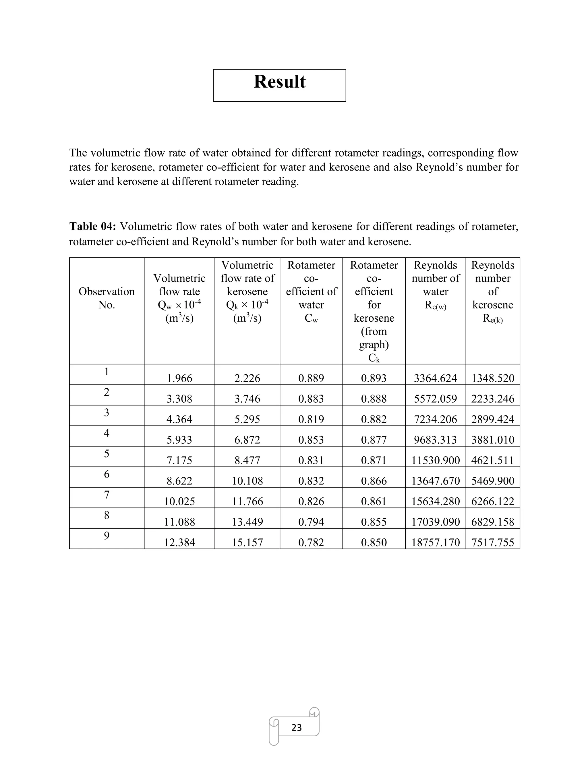
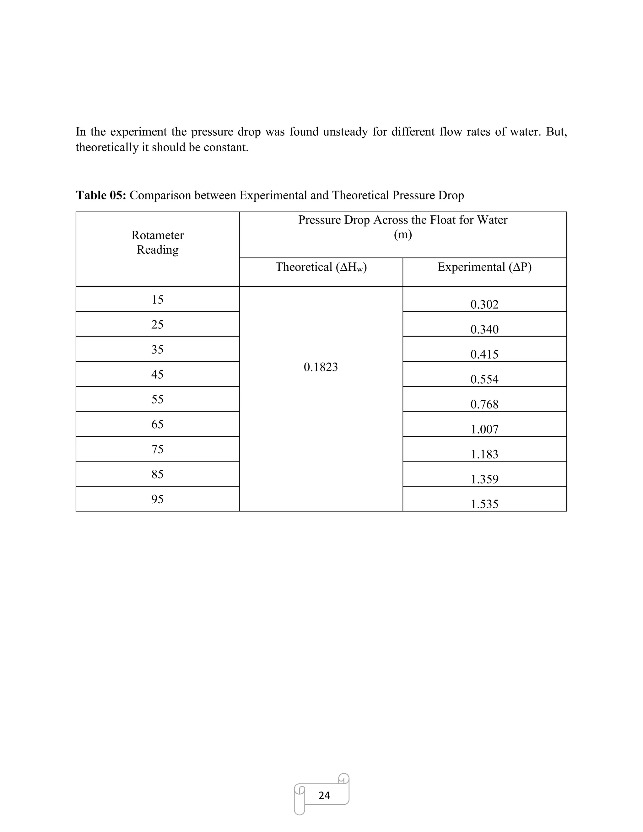
The study calibrated a rotameter for measuring the flow rates of multiple fluids. To calibrate the rotameter, the volumetric flow rate of water was measured for different rotameter readings by collecting water in a bucket over timed intervals. From the water flow rate readings, the rotameter coefficient (C) and Reynolds number (Re) were calculated and plotted against each other to obtain the calibration curve, which allows determining the flow rates of other fluids like kerosene from their properties and the rotameter reading.

1. 1/8/2018
STUDY OF A ROTAMETER
AND ITS CALIBRATION FOR
MULTIPLE FLUIDS
Fahim Shahriar Sakib
ID: 1502043
Level-2, Term-2
Group No: 03(A2)
Partners’ ID: 1502041
1502042
1502044
1502045
Department of Chemical Engineering, BUET
SUBMITTED TO
Oindrila Hossain
Lecturer
Department of Chemical
Engineering, BUET

2. 1
Acknowledgement
The work (Study of a rotameter and its calibration for multiple fluids) reported in this
paper has been carried the Fluid Mechanics Laboratory of Chemical Engineering Department,
Bangladesh University of Engineering and Technology, during the period September,2017.
I, hereby acknowledge my deep indebtedness to my teachers specially Oindrila Hossain
madam and for her continuous guidance, constructive suggestions, friendly behavior. During the
experiment, our instructors and the lab Assistant were always helpful to us. It gave me great
satisfaction to think me my teachers are always with us. I am also grateful to them for providing
me with the opportunity to do the report in a relatively independent manner. I also thank my lab
partners for helping hand.
Author Date: 08 January, 2018
Fahim Shahriar Sakib
ID: 1502043

3. 2
Forwarding letter
08 January, 2018
To
Oindrila Hossain
Lecturer
Department of Chemical Engineering, BUET.
Dhaka-1000.
Subject: Submission of report on “Study of a rotameter and its calibration for multiple fluids”
Dear Madam,
I am gladly informing you that I have completed the report on “Study of a rotameter and its
calibration for multiple fluids”. To submit this report in time, I had been busy in last few days.
Though it’s a time-consuming work, I am thanking you for this because to prepare this report, I
browsed internet, read many books which enlarged my knowledge about Rotameter. Being a
student of chemical engineering, it is so important for me. I would like to thank you for the
valuable instructions and guidelines that helped me greatly to prepare this report. I also would like
thank the instructors for their valuable instructions and great co-operation and my friends who
helped me to make it perfect one.
I hope, the information of this report will fulfill your expectation.
Yours faithfully,
Fahim Shahriar Sakib
ID: 1502043

4. 3
SUMMARY
Flow measurement is very important to any chemical process. There are many ways to measure
the flow rate of any fluids. One of the measuring instrument is Rotameter. It consists essentially
of a plummet, which is free to move vertically. It is slightly tapered with the small and down. The
fluid enters the lower end of the tube and causes the plummet to rise until the annular area between
the plummet and the wall of the tube is such that the pressure drop across this construction is just
enough to support the plummet. In glass tube, the float indicates the rates of flow. The float height
in the tube that is proportional to fluid flow rate. In this experiment, we will study Rotameter and
calibrate it for various fluids. Calibration means nothing but the relationship between volumetric
flow rate vs Rotameter reading. To calibrate rotameter, the volumetric flow rate of water for some
certain readings was measured. From the readings, C and Re/C are calculated and plotted in a
graph. This plot is ideal for a rotameter. Then the volumetric flow rate was calculated. Finally,
volumetric flow rate vs. Rotameter reading curve was plotted. The curve is linear, because
volumetric flow rate of any fluid is proportional to rotameter reading. The rotameter reading differs
from 15 to 95. The volumetric flow rates of water differ from 1.97×10-4
m3
to 12.38×10-4
m3
and
the volumetric flow rates of kerosene differ from 2.23×10-4
m3
to 15.15×10-4
m3
.

5. 4
List of Contents
Topic Page
Acknowledgement …. …. … … … … .. ……………….. …. …. …. …. …. .. ….. 01
Forwarding letter………………………………………..…………………………… 02
Summary ………………………………………………..………………………...… 03
1. Introduction ……………………………………………………………………. 06
2. Theory ……………………………………………………………………......... 07
3. Apparatus …………………………………………………………………........ 11
4. Experimental setup ……………………………………………………………. 12
5. Experimental procedure ……………………………………………………….. 13
6. Data table ……………………………………………………………………… 14
6.1. Observed data ………………………...………………………………….... 14
6.2. Calculated data ……………………………………………………….…… 15
7. Sample Calculation……………………………………………………………. 17
8. Graphical Representation……………………………………………………… 20
9. Results…………………………………………………………………….…… 23
10. Discussion……………………………………………………………………... 25
11. Conclusion ……………………………………………………………………. 26
References ...………………………………………………………………………... 27
Nomenclature ………………………………………………………………………. 28

6. 5
List of Illustrations
Figure 01: Forces on a rotameter ………………………………………………………….… (07)
Figure 02: Rotameter Tube and Float …..……….…………….………………………..…… (09)
Figure 03: Experimental setup for calibration of a rotameter ……….....……………………. (12)
Figure 04: Rotameter co-efficient vs (Reynolds number/ Rotameter co-efficient) for water .. (20)
Figure 05: Rotameter co-efficient vs (Reynolds number/co-efficient) for kerosene ………… (21)
Figure 06: Volumetric flow rate vs Rotameter reading for both water and kerosene ……….. (22)
List of tables
Table 01: Rotameter and manometer reading at different time intervals ……………………… (14)
Table 02: Calculated volumetric flow rate, velocity, equivalent diameter, diameter at the level of
float and annulus area …………………………………………………………….… (16)
Table 03: Calculated Reynolds number, rotameter coefficient and volumetric flow rate of
kerosene ……………………………………...………….…………………….…... (16)
Table 04: Results ………………………………..…………………………………………… (23)
Table 05: Results …………………………..………………………………………………… (24)
Table 06: List of symbols used throughout the report ……………………………………….. (28)

7. 6
INTRODUCTION
The chemical, paper, and minerals processing industries and pollution control facilities all have
various fluid streams entering and leaving different processes. In order to control these processes
and calculate material mass balance properly, it is important to calculate the flow rate of the fluid
stream properly. There are many ways and on basis of these ways many instruments are used to
measure of the flow rate of the fluid. The most common flow measurement instruments are the
variable head meters and the variable area meter. The variable area meter works on the principle
of varying area of flow at different flow rates so as to produce a constant pressure head differential.
One of the variable area meter is ‘Rotameter’. This is commonly used for any fluids especially for
high viscous fluids. A rotameter consists of a gradually tapered glass tube mounted vertically in a
frame with the large end up. The fluid flows up through the tube and suspends freely a float. As
the flow varies, the float rises or falls thus varying the area of the annular space between it and the
tube, so that the head loss across this annulus is equal to the weight of the float. The tube is marked
in divisions and the reading of the meter is taken from the scale reading and the reading edge of
the float, which is taken at the largest cross section of the float.
We can’t measure the flow rate of the fluid stream by only rotameter reading. We have to use a
calibration chart. Calibration means nothing but the relationship between the rotameter reading
and the flow rate. Floats are constructed of metals of various densities, glass or plastic. They also
may have various shapes and proportions for different applications.
In this experiment the calibration has to be done for different fluids e.g. water, kerosene etc. The
purpose of the calibration process is to plot a calibration curve for one fluid. The principal step of
the calibration process is to plot (rotameter co-efficient vs. Re/C) for the rotameter which is
independent of fluids. From this curve, for any fluids calibration curve can be drawn from the
density and viscosity data of that fluid.

8. 7
THEORY
Devices used to measure flow of fluids fall into two categories (variable pressure meters of variable
area meters). The rotameter is a flow meter falling into the latter category. It consists of a plummet
of float which is forced to move inside a tapered glass tube. The tube is graduated to give the flow
rater reading. The fluid stream passes through the glass tube with the float remaining suspended
by the upward movement of the fluid. The rate of flow is indicated by the equilibrium height of
the float. For a rotameter with given dimensions and float, the C vs Re/C curve is constant
regardless of the fluid used, thus by plotting C vs Re/C curve for one fluid we can calibrate it for
multiple fluids.
Since at equilibrium the float is stationary at any given flow rate, the downward and upward forces
acting upon it must be equal. The downward force equals to Vf(ρf - ρ) and the upward force on the
plummet is Af (P1-P2).
Here,
• Vf = Volume of the float, (ft3
)
• ρf = density of the, (lb/ft3
)
• ρ = density of the fluid, (lb/ft3
)
• Af = cross sectional area of the float at its widest part, (ft2
)
• P1= upward pressure on the float, (lb/ft2
)
• P2 = downward pressure on the float, (lb/ft2
)
Figure 01: Forces on a rotameter

9. 8
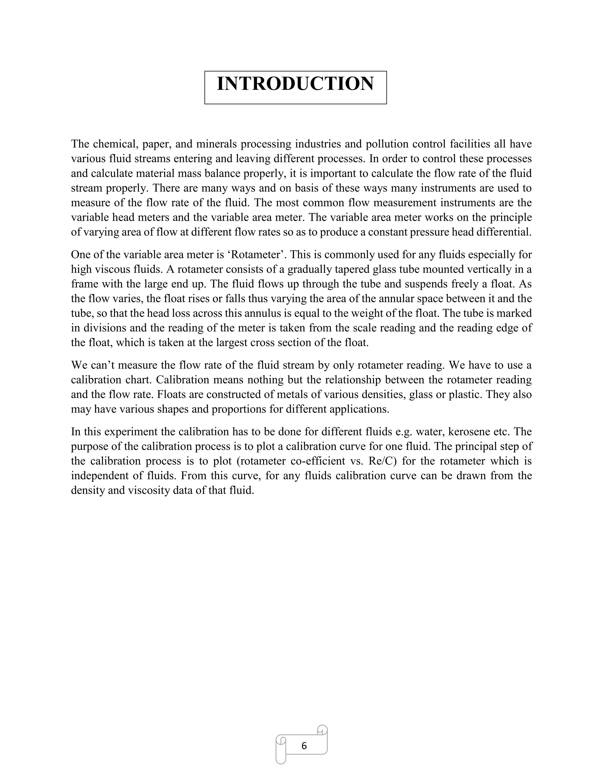
Head loss across the annulus is seen to depend on float and liquid characteristics only. Since a
rotameter can be considered an orifice meter with variable aperture. The flow equation for an
orifice is therefore applicable for a rotameter.
V = C √2𝑔 𝐻 ……………………………. (1)
Where,
V =average linear velocity of the fluid through the annulus, ft/sec
C = rotameter co-efficient, dimensionless
g = acceleration due to gravity
H = Net head loss across the annulus = Vf (
 𝑓−
𝐴 𝑓
)
Now, v = Q/Ao (ft/sec).
Where Q = volumetric flow rate, (ft3
/sec.)
Ao = annulus cross sectional between float and tube, ft2
V = Q/Ao = C √2𝑔 𝐻 = C√2𝑔Vf(
 𝑓−
𝐴 𝑓
)
Solving for C, we have
C =
𝑄
𝐴 𝑜√[
2𝑔𝑉 𝑓( 𝑓−)
𝐴 𝑓
]
=
𝑄
𝐴 𝑜√(2𝑔 𝐻)
……………………. (2)
With known Q for water (Qw), known ΔHw and known Ao, for a corresponding rotameter reading,
we can thus find C using (2).
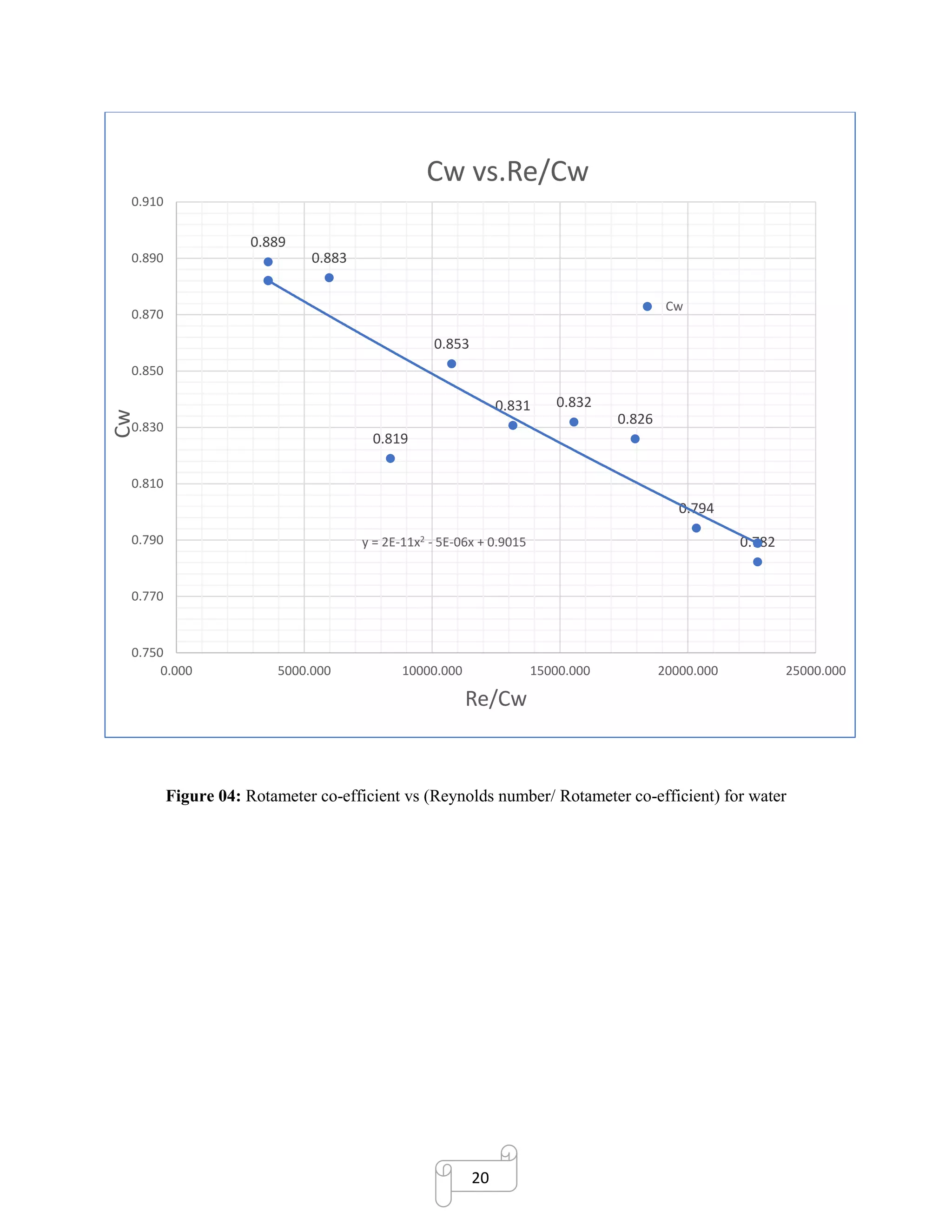
Thus, we can find a series of C values for various rotameter readings. Also, we can find Re
(Reynolds’ number) at these rotameter readings. This helps us to plot C vs Re/C curve
(Calibration curve).

10. 9
D2
Flow of fluid
Df R
Float
D1
Dt
Figure 02: Rotameter Tube and Float
Now, Re =
𝐷 𝑒𝑞 𝑣 

……………………………. (3)
on dividing equations (3) by (1), we get
Re/C = Deq


√2𝑔 𝐻 ……………………………. (4)
In equation (4) Re/C is determined by rotameter reading while the other terms are dependent
only on float and fluid properties.
Calculation of Df and Deq
Equivalent diameter, Deq =
4𝐴 𝑜
(𝑤𝑒𝑡𝑡𝑒𝑑 𝑝𝑒𝑟𝑖𝑚𝑒𝑡𝑒𝑟)
= Dt - Df
A0
Df

11. 10
Where,
• Dt = diameter of rotameter tube at the maximum cross sectional of float, (ft)
(Develop an equation relating Dt and rotameter reading, R)
• Df = maximum diameter of float, (ft)
And Ao =
(𝐷𝑡
2
−𝐷 𝑓
2
)
4
Calculation of Q2 from Q1:
Let Q1 is the flow rate of water and Q2 is the flow rate of oil at a particular reading of the
rotameter. Like equation (2), equation for Q1 and Q2 are then set up as flows,
Q1= C1Ao √2𝑔 𝐻1
Q2= C2Ao √2𝑔 𝐻2
Let the calibration curve look as follows:
C
Re/C
For any rotameter reading the corresponding C/Re for any other fluid i.e. (C/Re)2 can be calculated.
The corresponding (C2) can be found from the above graph.
Dividing the above two equations we get
𝑄2
𝑄1
=
𝐶2√ 𝐻2
𝐶1√ 𝐻1
………………………………. (5)
For finding the flow rate of kerosene from water we may write
𝑄 𝑘
𝑄 𝑤
=
𝐶 𝑘√ 𝐻 𝑘
𝐶 𝑤√ 𝐻 𝑤
Where, Hk = Vf(
 𝑓− 𝑘
𝐴 𝑓 𝑘
)

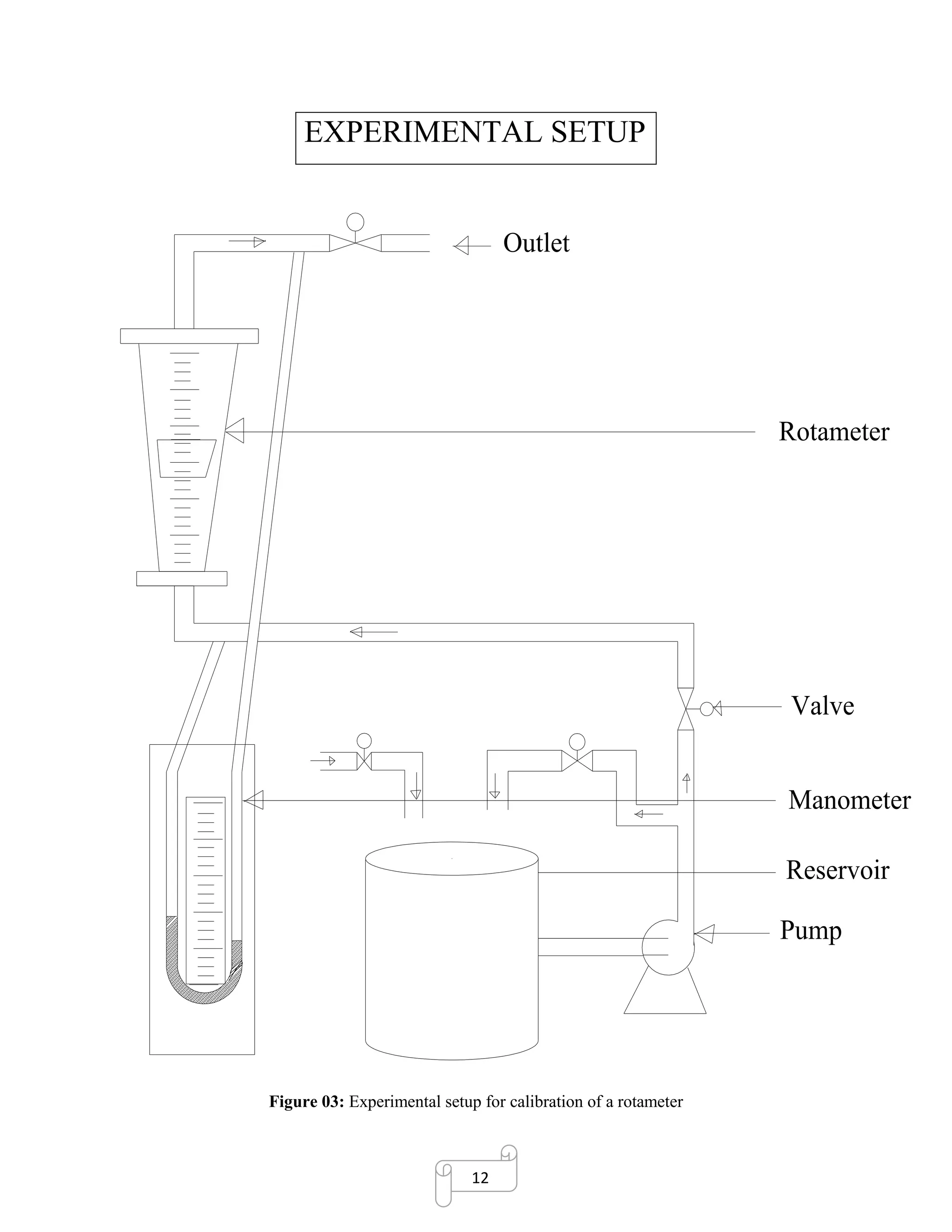
12. 11
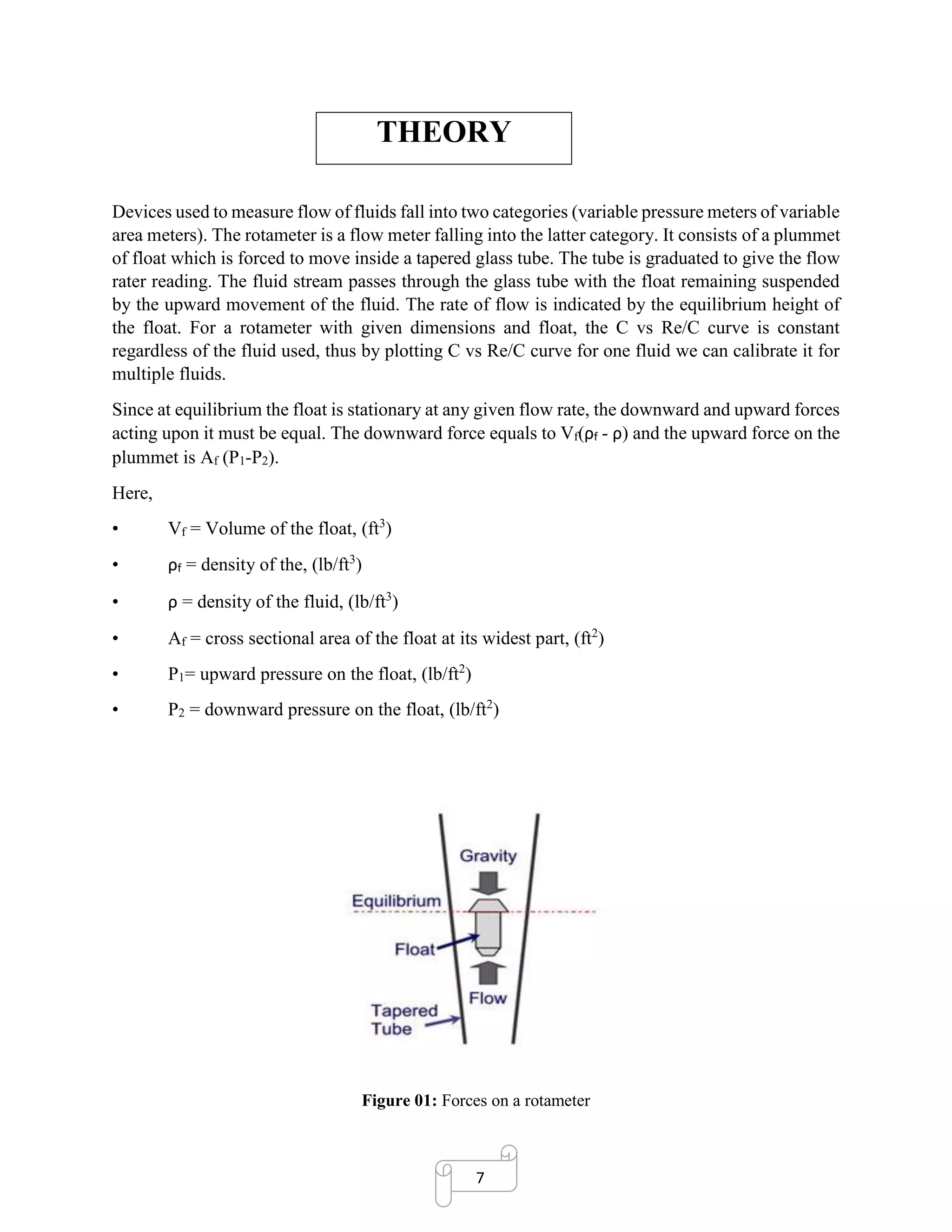
APPARATUS
1. Rotameter – [Rotameter is a typical variable area meter consists of gradually tapered glass
mounted vertically in a frame with the large end up. Fluid flows upward through the
tapered tube and suspends freely a float (which is submerged in the fluid) Float is the
indicating element, and the greater the flow rate, the higher the float rides in the tube. The
float is shaped so that it rotates axially as the fluid passes. Floats are made in many different
shapes, with spheres and spherical ellipses being the most common. The tube is marked in
divisions, and the reading of the meter is obtained from the scale reading at the reading
edge of the float, which is taken at the largest cross section of the float.]
2. Manometer – [A meter which is used for measuring the pressure drop between two points.
It is normally ‘U’ shaped. There is a manometric fluid from which we can measure the
pressure difference. There are different types of manometer. But here, we used ‘U’ shaped
and two ways open manometer.]
3. Bucket – [A little reservoir which is used for measuring mass flow rate of a fluid. In a
period of time, we filled water in bucket and measured the mass flow rate.]
4. Stopwatch – [It is used for measuring mass flow rate. It is used for limiting the time
interval.]
5. Weighing machine – [we used it for measuring the mass of water which is taken in a time
period.]
6. Tank – [The water is reserved in tank.]
7. Pump – [It is used for flowing the water through the rotameter for proceeding the
experiment]

13. 12
EXPERIMENTAL SETUP
Outlet
Pump
Valve
Manometer
Rotameter
Reservoir
Figure 03: Experimental setup for calibration of a rotameter

14. 13
EXPERIMENTAL PROCEDURE
The experimental procedure is followed in these ways:
1. We took the value of the density of the float (Sf) and volume of the float (Vf) from the
rotameter manual.
2. We measured the float diameter at its widest part and the inside diameters of the rotameter
tube at both ends.
3. Then intermediate diameters are calculated by assuming a linear relationship.
4. The volumetric flow rate of water is controlled by a valve.
5. Pressure drop readings with float are then taken for different flow rates.
Then the calculation steps were done to calibrate the rotameter for different fluids, e.g. kerosene.

15. 14
DATA TABLE
Observed Data:
Room temperature = 230 C
Temperature of the water = 22.5o
C
Table 01: Observed data for Rotameter and manometer reading, manometer reading difference at
different time intervals.
No. of
observation
Time
(sec)
Rotameter
Reading
Weight of
Water
(Kg)
Manometer
Reading
(cm) Difference
(cm)
Left Right
1 5.1 15 1.00 31.9 29.5 2.4
2 5.0 25 1.65 32.1 29.4 2.7
3 5.1 35 2.22 32.4 29.1 3.3
4 4.9 45 2.90 33.0 28.6 4.4
5 5.1 55 3.65 34.0 27.9 6.1
6 5.0 65 4.30 35.0 27.0 8.0
7 5.0 75 5.00 35.7 26.3 9.4
8 5.0 85 5.53 36.5 25.7 10.8
9 5.1 95 6.30 37.2 25.0 12.2

16. 15
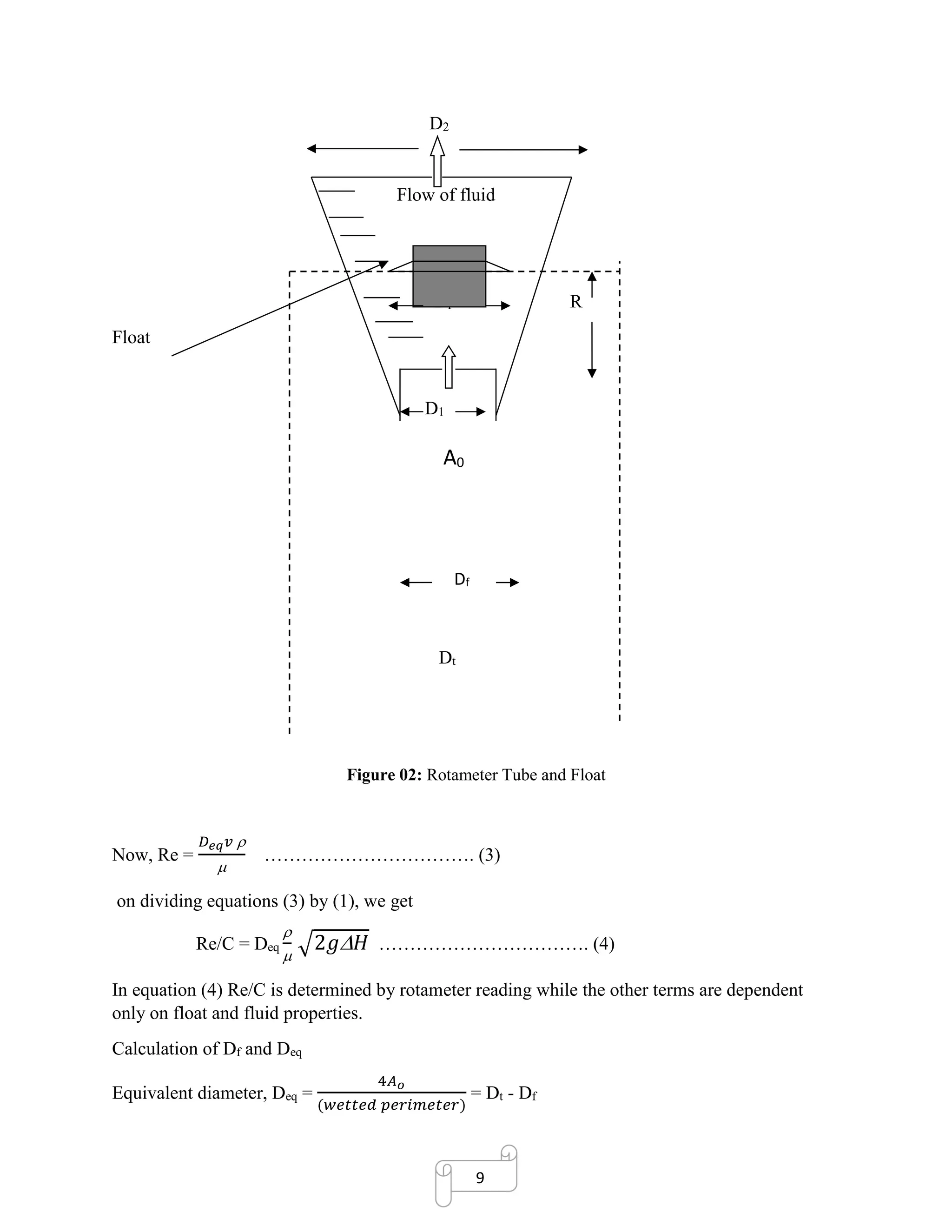
Calculated Data:
Equipment data
Diameter of rotameter tube at lower end, D1= 1.5 inch = 3.81×10-2
m
Diameter of rotameter tube at upper end, D2= 2.0 inch = 5.08×10-2
m
Total length of rotameter tube, L=100 divisions
Maximum float diameter, Df= 1.5 inch= 3.81×10-2
m
Volume of the float, Vf= 1.077×10-3
ft3
= 3.05×10-5
m3
Density of the float, ρf = 486.93 lbm/ft3
=7804.64 kg/m3
Collected data
At 22.5o
C
Density of water, ρw = 997.6 Kg/m3
Viscosity of water, µw = 8.96×10-4
Ns/m-2
[By interpolation (Ref: Daugherty, Franzini
& Finnemore, Fluid Mechanics with
Engineering Application, SI metric edition,
Page-591)]
At 200
C
Density of kerosene ρk= 808 kg/m3
Viscosity of kerosene µk = 1.92×10-3
Ns/m2
Specific weight of kerosene γk=810 kN/m3
[Ref: Daugherty, Franzini & Finnemore,
Fluid Mechanics with Engineering
Application, SI metric edition, Page-573]

17. 16
Table 02: Data table of mass flow rate, volumetric flow rate, Diameter of rotameter at the level of float,
annulus area, equivalent diameter & velocity.
Observation
No.
Mass flow
rate of
water
M
(kg/s)
Volumetric
flow rate
Qw 10-4
(m3
/s)
Diameter of
the
rotameter at
the level of
float
Dt 10-2.
(m)
Annulus
Area
A0  10-4
(m2
)
Equivalent
diameter
Deq10-3
(m)
Velocity
V
(ms-2
)
1 0.20 1.97 4.00 1.17 1.91 1.68
2 0.33 3.31 4.13 1.98 3.18 1.67
3 0.44 4.36 4.25 2.82 4.45 1.55
4 0.59 5.93 4.38 3.68 5.72 1.61
5 0.72 7.17 4.51 4.56 6.99 1.57
6 0.86 8.62 4.64 5.48 8.26 1.57
7 1.00 10.03 4.76 6.41 9.53 1.56
8 1.11 11.09 4.89 7.38 10.80 1.50
9 1.24 12.38 5.02 8.36 12.07 1.48
Table 03: Data table of Reynold number, Rotameter Coefficient for Water & Kerosene and Volumetric
Flow rate of Kerosene.
Pressure Drop m Reynolds
number of
water
Re
Rotameter
co-
efficient
of water
Cw
(Re/Cw)
For water
(Re/Ck)
For
kerosene
Rotameter
co-
efficient
for
kerosene
(from
graph)
Ck
Volumetric
flow rate of
kerosene
Qk × 10-4
(m3
/s)Water
wH
Kerosene
kH
0.183 0.232
3364.624 0.889 3588.757 1709.195 0.893 2.226
5572.059 0.883 5981.261 2848.658 0.888 3.746
7234.206 0.819 8373.765 3988.121 0.882 5.295
9683.313 0.853 10766.270 5127.584 0.877 6.872
11530.900 0.831 13158.774 6267.047 0.871 8.477
13647.670 0.832 15551.279 7406.51 0.866 10.108
15634.280 0.826 17943.783 8545.973 0.861 11.766
17039.090 0.794 20336.287 9685.436 0.855 13.449
18757.170 0.782 22728.792 10824.9 0.850 15.157

18. 17
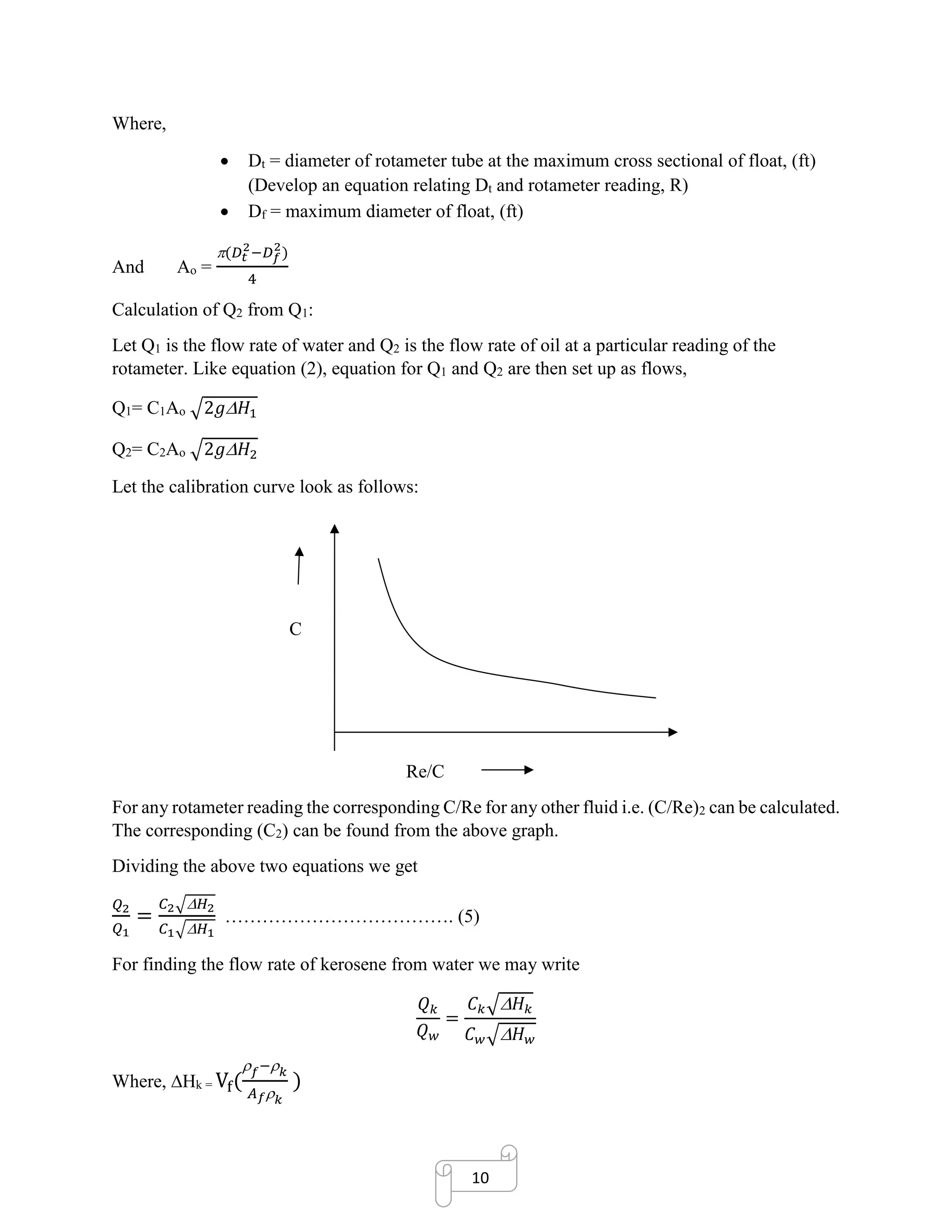
SAMPLE CALCULATION
Sample calculation for the ninth (8th
) observation is given below:
Flow Rates Calculation:
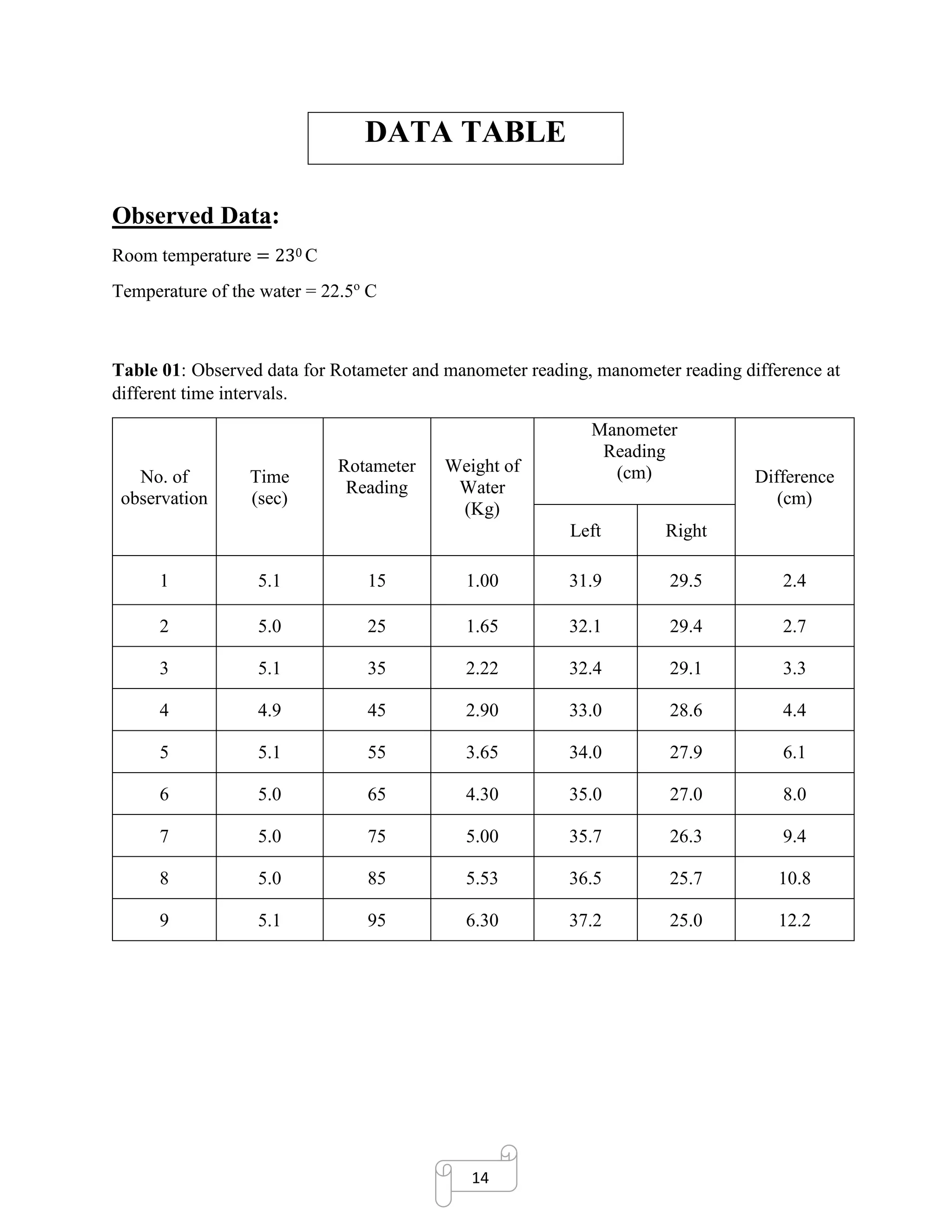
▪ Mass of empty bucket as reference
▪ Mass of water, m = 5.53kg
▪ Time, t = 5.00 s
▪ Mass flow rate, M =
5.53 𝑘𝑔
5.00 𝑠
= 1.11 kg / s
▪ Density of the water at 22.50
C ρw = 997.6 kg/m3
▪ Volumetric flow rate, Qw =
𝑚

=
1.11
997.6
m3
/s = 11.09 × 10-4
m3
/s
Calculation of Rotameter Data:
✓ Diameter of rotameter tube at lower end, D1= 1.5 inch = (1.5 × 0.0254) = 0.0381 m
✓ Diameter of rotameter tube at upper end, D2= 2.0 inch = (2.0 × 0.0254) = 0.0508 m
✓ Maximum float diameter, Df= 1.5 inch= 3.81×10-2
m
✓ Volume of the float, Vf= 1.077×10-3
ft3
= [(1.077 × 10−3)𝑓𝑡3
× 0.0283
𝑚3
𝑓𝑡3
]
= 3.05×10-5
m3
✓ Density of the float, ρf = 486.93 lbm/ft3
= [(486.93
𝑙𝑏 𝑚
𝑓𝑡3
× 0.4536
𝑘𝑔
𝑙𝑏 𝑚
) ÷ 0.0283
𝑚3
𝑓𝑡3
]
=7804.64 kg/m3
✓ Area of the float, Af =
Df
2
4
=
3.1416 x (0.0381)2
4
= 1.14 × 10-3
m2
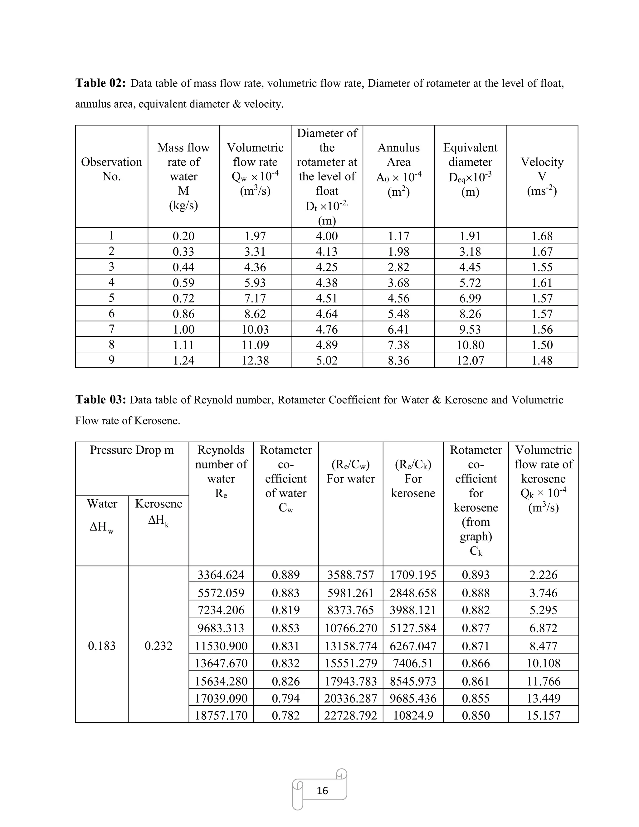
✓ Diameter of rotameter tube at the maximum cross section of float,
Dt = D1 + (D2 − D1) ×
R
100
= 0.0381 + (0.0508 − 0.0381) ×
85
100
m = 0.0489 m
✓ Annulus cross sectional area between float and tube, Ao =
(𝐷𝑡
2
−𝐷 𝑓
2
)
4
=

4
× [(0.0489)2
− (0.0381)2
] = 7.38 × 10-4
m2
✓ Equivalent diameter, Deq = Dt - Df = (0.0489 − 0.0381) = 0.0108 m

19. 18
Calculation of Rotameter Co-efficient for Water:
➢ Net head loss across the annulus, Hw = Vf (
 𝑓− 𝑤
𝐴 𝑓 𝑤
)
= [3.05 × 10−5
(
7804.64−997.6
1.14×10−3×997.6
)] = 0.1826 m
➢ Rotameter co-efficient for water, Cw =
𝑄 𝑤
𝐴 𝑜√2𝑔 𝐻 𝑤
=
11.09 × 10−4
8.36𝑥10−4√2×9.8×0.1826
= 0.794
➢ Viscosity of water, µw = 8.96×10-4
Ns/m-2
[By interpolation (Ref: Daugherty, Franzini & Finnemore, Fluid
Mechanics with Engineering Application, SI metric edition, Page-591)]
From equation (4)
• Re/C = 𝐷𝑒𝑞


√2𝑔 𝐻 = 10.80 × 10−3
×
997.6
8.96×10−4
× √2 × 9.81 × 0.1826 = 20336.287
Calculation of Rotameter Co-efficient for Kerosene:
At 200
C
Density of kerosene ρk= 808 kg/m3
Viscosity of kerosene µk = 1.92×10-3
Ns/m2
[Ref: Daugherty, Franzini & Finnemore,
Fluid Mechanics with Engineering
Application, SI metric edition, Page-573]
➢ Net head loss across the annulus, Hk = Vf (
 𝑓− 𝑘
𝐴 𝑓 𝑘
) = [3.05 × 10−5
(
7804.64−808
1.14×10−3×808
)]
= 0.232 m
• For Kerosene, Re/C = 𝐷𝑒𝑞
𝜌 𝑘

√2𝑔𝐻 = 10.80 × 10−3
×
808
1.92×10−3
× √2 × 9.81 × 0.232
= 9685.436
From Figure 04, the value of rotameter coefficient for Kerosene, Ck= 0.855 when Re/C = 9685.436

20. 19
Calculation for Volumetric Flow Rate for Kerosene:
𝑄 𝑘
𝑄 𝑤
=
𝐶 𝑘√ 𝐻 𝑘
𝐶 𝑤√ 𝐻 𝑤
 Qk = Qw ×
𝐶 𝑘√ 𝐻 𝑘
𝐶 𝑤√ 𝐻 𝑤
= 12.38 x 10-4
×
0.855√0.2321
0.794√0.1824
= 13.449 × 10-4
m3
/s
Calculation of Experimental Pressure Drop:
Density of Mercury at 200
C, Hg = 13550 kg/m3
[Ref: Daugherty, Franzini & Finnemore,
Fluid Mechanics with Engineering
Application, SI metric edition, Page-573]
➢ Experimental pressure drops, P = R (
 𝐻𝑔− 𝑤
 𝑤
) = 0.108 x (
13550−997.6
997.6
)
= 1.359 m

21. 20
Figure 04: Rotameter co-efficient vs (Reynolds number/ Rotameter co-efficient) for water
0.889
0.883
0.819
0.853
0.831 0.832
0.826
0.794
0.782y = 2E-11x2 - 5E-06x + 0.9015
0.750
0.770
0.790
0.810
0.830
0.850
0.870
0.890
0.910
0.000 5000.000 10000.000 15000.000 20000.000 25000.000
Cw
Re/Cw
Cw vs.Re/Cw
Cw

22. 21
Figure 05: Rotameter co-efficient vs (Reynolds number/ Rotameter co-efficient) for kerosene
0.893
0.888
0.882
0.877
0.871
0.866
0.861
0.855
0.850
0.845
0.850
0.855
0.860
0.865
0.870
0.875
0.880
0.885
0.890
0.895
0.900
0 2000 4000 6000 8000 10000 12000
Ck
Re/Ck
Ck vs.Re/Ck
Ck

23. 22
Figure 06: Volumetric flow rate vs Rotameter reading for both water and kerosene
0.00E+00
2.00E-04
4.00E-04
6.00E-04
8.00E-04
1.00E-03
1.20E-03
1.40E-03
1.60E-03
0 10 20 30 40 50 60 70 80 90 100
VolumetricFlowRate
Rotameter Reading
Volumetric Flow Rate vs. Rotameter Reading
Qw Qk

24. 23
Result
The volumetric flow rate of water obtained for different rotameter readings, corresponding flow
rates for kerosene, rotameter co-efficient for water and kerosene and also Reynold’s number for
water and kerosene at different rotameter reading.
Table 04: Volumetric flow rates of both water and kerosene for different readings of rotameter,
rotameter co-efficient and Reynold’s number for both water and kerosene.
Observation
No.
Volumetric
flow rate
Qw 10-4
(m3
/s)
Volumetric
flow rate of
kerosene
Qk × 10-4
(m3
/s)
Rotameter
co-
efficient of
water
Cw
Rotameter
co-
efficient
for
kerosene
(from
graph)
Ck
Reynolds
number of
water
Re(w)
Reynolds
number
of
kerosene
Re(k)
1
1.966 2.226 0.889 0.893 3364.624 1348.520
2
3.308 3.746 0.883 0.888 5572.059 2233.246
3
4.364 5.295 0.819 0.882 7234.206 2899.424
4
5.933 6.872 0.853 0.877 9683.313 3881.010
5
7.175 8.477 0.831 0.871 11530.900 4621.511
6
8.622 10.108 0.832 0.866 13647.670 5469.900
7
10.025 11.766 0.826 0.861 15634.280 6266.122
8
11.088 13.449 0.794 0.855 17039.090 6829.158
9
12.384 15.157 0.782 0.850 18757.170 7517.755

25. 24
In the experiment the pressure drop was found unsteady for different flow rates of water. But,
theoretically it should be constant.
Table 05: Comparison between Experimental and Theoretical Pressure Drop
Rotameter
Reading
Pressure Drop Across the Float for Water
(m)
Theoretical (Hw) Experimental (P)
15
0.1823
0.302
25 0.340
35 0.415
45 0.554
55 0.768
65 1.007
75 1.183
85 1.359
95 1.535

26. 25
DISCUSSION
1. The curve for volumetric flow rates vs. rotameter readings was drawn for water and
kerosene both of the curves. From graph we found a straight line. But the slope of the line
for kerosene is greater than that of the slope of line for water. The only reason behind this
incident is the density of kerosene is less than that of the density of water and the volumetric
flow rate of kerosene for the same rotameter reading is larger than the flow rate of water.
2. The manometer we used was slightly defected. The mercury level was fluctuating fast. We
ignored this defect by taking measurements quickly.
3. There was some leakage in pipe fittings. So, our result is not totally accurate.
4. The rotameter coefficient is a function of Reynolds number. The curve of rotameter co-
efficient vs (Reynolds number/rotameter co-efficient) is not independent of fluid. But if
the fluid density is negligible in comparison with float density, it may be considered as
independent of fluids. This curve also differs with shape and nature of rotameter float.
5. The head losses for water and kerosene are theoretically constant values. Theoretically we
found it 0.182 m and 0.231m. In this experiment, the manometer readings were not
constant. Practically the head loss was proportional to the flow rates. There are also some
minor losses like: (Entrance loss, Expansion loss, Contraction loss, Exit loss). These
losses are occurred in the rotameter tube. These were not considered. The actual head loss
was affected by these losses.
6. The known fluid must be transparent so that the operator can see the position of the float.
It is needed to gain correct value.
7. These drawbacks can be modified by using rotameter which is made from opaque tube to
withstand higher pressures. The position of the float is sensed from outside of the tube by
an electromagnetic means and the flow rate is indicated on a gage. Color fluids can also be
used in this rotameter.

27. 26
CONCLUSION
After performing the experiment, these major conclusions can be drawn: -
1. Rotameter is a variable area meter. Head loss across it is very little. It May be constructed
from a variety of materials and cover a wide range of temperatures and pressures. Easily
read, installed, and maintained. But it can’t be used horizontally.
2. This experiment was an introduction to the variable area meters used in chemical processes.
This can help a student to know about the common flow meter and its working principal.
A student could know about the calibration process of a flow measuring device also, which
is very much important for a chemical engineer.
3. When fluid flows at ideal (frictionless pipe, incompressible, ideal fluid) rate the pressure
drop across the rotameter become constant.
4. After generating the calibration curve of the rotameter, it can be used for measuring
multiple fluids flow rates.

28. 27
REFERENCES
✓ Daugherty, Franzini & Finnemore, Fluid Mechanics with Engineering Application, SI
metric edition, Page. 571-573
✓ Mott, Robert L.: applied fluid mechanics, 5th ed., Prentice Hall New Jersey, p. 448-449
(2000)
✓ Sensors, Flowmeter, Variable Area, 06 January, 2018, www.efunda.com
✓ Rotameter, 06 January, 2018, www.wikipedia.com
✓ Rotameter, 06 January, 2018, www.omega.com

29. 28
NOMENCLAUTURE
Table 06: List of symbols used throughout the report
Symbols Name Unit
Af Cross-sectional area of the float at its widest part ft2
, m2
Ao Annular cross-sectional area ft2
, m2
C Rotameter co-efficient Dimensionless
D1 Diameter of the rotameter tube at lower end ft, m
D2 Diameter of the rotameter tube at upper end ft, m
Deq Equivalent diameter ft, m
Df Maximum diameter of float ft, m
Dt Diameter of the rotameter tube at the maximum
cross section of float
ft, m
g Acceleration due to gravity ft/s2
,m/s2
ΔH Net head loss ft, m
P Pressure head ft, m
M Mass flow rate kg/s
Q Volumetric flow rate ft3
/s, m3
/s
Re Reynolds’ number Dimensionless
V Volume ft3
, m3
 Density lbm/ft3
, kg/m3
 Viscosity lb/ft.s , kg/m.s

30. 29
Name: Fahim Shahriar Sakib
Student Number: 1502043
Sections and % marks allocated Marks
Summary (10%)
Introduction and theory (15%)
Experimental work (15%)
Results and discussions (25%)
Reference and nomenclature (5%)
Quality of figures (10%)
Quality of tables (10%)
Overall presentation (10%)
Total (100%)