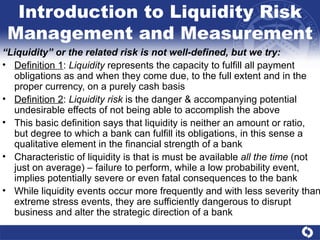
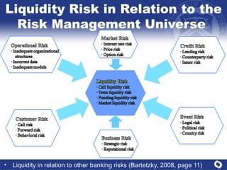
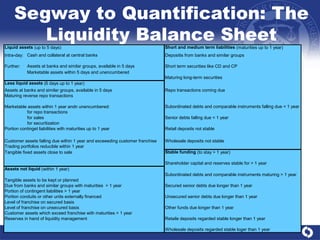
Quantitative Measurement and Management of Liquidity Risk in a Banking Context Michael Jacobs, PhD, CFA Senior Financial Economist Credit Risk Analysis Division / U.S. Office of the Comptroller of the Currency G.A.R.P. 13 th  Annual Risk Management Convention February 2012 The views expressed herein are those of the authors and do not necessarily represent the views of the Office of the Comptroller of the Currency or the Department of the Treasury.
Outline Introduction to Liquidity Risk Management and Measurement Conceptual Considerations in Liquidity Risk Quantitative Frameworks for Managing Liquidity Risk  A Simple Model for Liquidity Risk An Option Theoretic Model for Liquidity Risk Summary of Findings
Introduction to Liquidity Risk Management and Measurement “ Liquidity” or the related risk is not well-defined, but we try: Definition 1 :  Liquidity  represents the capacity to fulfill all payment obligations as and when they come due, to the full extent and in the proper currency, on a purely cash basis Definition 2 :  Liquidity risk  is the danger & accompanying potential undesirable effects of not being able to accomplish the above This basic definition says that liquidity is neither an amount or ratio,  but degree to which a bank can fulfill its obligations, in this sense a qualitative element in the financial strength of a bank Characteristic of liquidity is that is must be available  all the time  (not just on average) – failure to perform, while a low probability event, implies potentially severe or even fatal consequences to the bank While liquidity events occur more frequently and with less severity than extreme stress events, they are sufficiently dangerous to disrupt business and alter the strategic direction of a bank
Introduction to Liquidity: Review of the Literature Knies (1876): stress the necessity for a cash buffer to bridge negative payment gaps between inflows and outflows where timing is uncertain Stutzel (1959, 1983): further discussions focusing primarily on basic considerations between liquidity and solvency New focus starting in mid-1990s on specific issue of liquidity risk management, mainly dealing with policy: Matz (2002), Zeranski (2005), Matz and Neu (2007), Bartetzky,Gruber and When (2008)  BCBS (2000, 2006, 2008): supervisory expectations & best practices for managing liquidity risk in financial institutions Quantitative frameworks: Fielder (2007), Hiedorn & Schamlz (2008), Reitz (2008) Duttweiler (2008): an holistic view of liquidity risk including quantitative methods (LaR & VaR)
Introduction to Liquidity:  Empirics and Stylized Facts * Proxies for risk types from quarterly financial data: credit = gross chargeoffs, operational = other non-interest expense, market = deviation in 4-quarter avg. trading revenues, interest rate = deviation in 4-quarter avg.  interest rate gap  (rate on deposits – loans), liquidity = deviation in 4-quarter avg.  liquidity gap  (loans-deposits)  Generally, this measure of liquidity risk exhibits positive and sometimes substantial correlation with other risk types * Source: Inanoglu, H., and Jacobs, Jr., M., 2009, Models for risk aggregation and sensitivity analysis: An application to bank economic capital, Journal of Risk and Financial Management, Vol. 2 (Summer), 118-189.
Introduction to Liquidity:  Empirical Evidence (continued) * Measure as ratio of liquid assets to total value of banking book Secular decline in 20 years going into recent crisis (except 1990 spike)  But now rapid & massive increase from depth to end of crisis?  * Source: Inanoglu, H., Jacobs, Jr., M. and R. Sickles, 2009, Analyzing bank efficiency: Are too-big-to-fail banks efficient?, Working paper, U.S. Office of the Comptroller of the Currency and Board of Governors of the Federal Reserve System.
Introduction to Liquidity Risk Management and Measurement The different types / meanings of liquidity and how they are related to each other (adapted from Bartetzky, 2008, page 9)
Liquidity Risk in Relation to the Risk Management Universe  Liquidity in relation to other banking risks (Bartetzky, 2008, page 11)
Conceptual Considerations: Stylized Facts Liquidity Risk Liquidity risk is generally thought to be a function of these Volume & tenor of assets as dictated by business policy Extent of tenor mismatch between assets & liabilities Stability of deposit base (eg, retail but short term & low volume) Optionality of bank assets (eg, undrawn commitments) Persistence of liquidity gap implies bank will have to get funding Terms of later financing not known in advance Even marketable assets can have different liquidity over time Willingness of market to fund depends on future bank state Bank financial state & perception depends upon inter-related data (eg, risk profile, solvency, profitability & trend) Bank’s forecast of self state & market perception of this are both risky & uncertain
Conceptual Considerations: How to Look at Liquidity Level of aggregation  includes several dimensions (amount, currency, time): advisable to maintain as detailed information as possible, even if not required by controllers or supervisors  Natural  (legal maturities) vs.  artificial  liquidity (shiftability & marketability-”business view”) & meeting customers’ needs & keep the franchise intact (not just surviving as a legal entity) Optionalities : apply not only to traded or OTC options but any bank commitment that puts the bank in a  position of an option seller exposed to unpredictable cash requirements The impact of  business policy  on liquidity: the need for a dynamic perspective & accounting vs. actual cash flows
Conceptual Considerations: Liquidity Risk & Other Risks Solvency  is the condition of sufficient capital to cover loss, a pre-condition but not sufficient for  liquidity  ( perceived  solvency can impact liquidity through investors/customers actions)  Liquidity vs. interest rate risk : it seems that they can be treated similarly with respect to gap analysis, but for a typical bank’s exposure it is unlikely that they form a predictable relationship E.g., prepayment: excess liquidity but reinvestment rate risk; CP line triggered: may have hedged rates with FRA but cash changes hands Liquidity vs. market liquidity risk : the ability to transform marketable assets into cash depends upon the breadth and depth of markets Depends on quality of issuer, market conditions & asset characteristics Ways to close the liquidity gap: international FIs-”asset driven model” vs. savings banks-”liability driven model” (but latter depends on behavior of lenders –”name” of institution & market)
Segway to Quantification: The Liquidity Balance Sheet
A Quantitative Framework for Managing Liquidity Risk Quantification of liquidity risk encompasses 4 key aspects: Behavior of the balance sheet structure under various circumstances Basic conditions required when applying a dynamic business perspective Forecasting the most likely liquidity gaps Linking these findings to liquidity policy 2 basic occurrences lead to increased liquidity risk: Asset: marketable assets loose quality or segment for which is conjested Liability: funding potential declines  Key components of a quantitative framework: Dynamic (planned & future developments need to be accounted for) Distinguish between normal & stressed environments Stressed circumstances can vary in quality Heterogeneity of impact upon particular banks Forward looking orientation
A Quantitative Framework for Managing Liquidity Risk (cont.) The  Liquidity Condition : the capability to fullfill all obligations as and when they come due in each currency & period: ELE t  is the  Expected Liquidity Exposure  in time t, the difference between expected negative and positive cash flow: LaR t α  is the  Liquidity-at-Risk , the deviations of in- and out-flows due to specific circumstances in period t, which like VaR focuses on the downside (i.e., danger of outflows exceeding inflows at some high confidence level 1- α ) CBC t  is the  Counter-Balancing Capacity  containing asset buffers which can be readily converted to liquidity (e.g., security sales, repos, collateralizations, etc.) or capability to renew existing contracts or new funds from other 3 rd  parties
We may state this equivalently as that CBC (e.g., asset reserves or funding slack) needs to exceed the sum of future exposures: CBC t  may be decomposed into the sum of asset (or funding) liquidity A, sale liquidity S and repo liquidity R (the latter 2 comprising balance sheet liquidity): We can adjust the formula for nostro balances kept  for payment purposes, which at day end if positive (negative) we will invested (borrow): Where FLE t  is  forward liquidity exposure  in period t Further adjustments to these are made to make this dynamic A Quantitative Framework for Managing Liquidity Risk (cont.)
Calculating ELE t  requires analysis of instruments with respect to amounts and timings of cash flows, which may be random Case 1 : time & amount determined (e.g., interest/principle payments on fixed rate funded loan commitments & deposits) Case 2 : time determined & amount random (e.g., dividends, floating legs of swap arrangements) Case 3 : time random & amount determined (e.g., loans with flexible payment agreements - PIKs) Case 4 : time & amount random (e.g., unfunded revolving commitments, savings deposits, own account trading exposure, clearing for 3 rd  parties) Adjustment 1: based upon the above analysis, decompose the ELE t  into deterministic and random components: F: floating (linked to market prices), V: virtual (not related to market or observable factors), H: hypothetical (new business, credit or operational risk events) A Quantitative Framework for Managing Liquidity Risk (cont.)
Firm can refinance in any period with any maturity but cannot repurchase bonds early If cannot roll-over debt then a restructuring cost of 16 (project’s low market liquidity increases this risk, a type of “funding illiquidity”) 2 strategies, short/long or long/short: while interest rate management gives no guidance, we can show that the former is optimal!  A 3 period project costing 100 & NPV =103 follows a binomial tree with probability ½ of up/down move Owner has no capital and must issue only zero coupon debt of maturity 1 or 2 Continuum of risk neutral bondholders who can invest in the risk-free asset at zero interest rate Quantitative Frameworks: A Simple Model Liquidity Risk 103 101 105 99 103 107 97 101 105 109 Period 3 Period 2 Period 1 Period 0 1a 1b 2a 2b 2c 3a 3b 3c 3d Short/Long Long/Short
Bonds sold at 1b will be at a discount to value 101 to compensate for default at 3d Therefore, in period 0 firm pursues short-long strategy, firm value is 103, bonds are worth 100 and there is equity of 3 This illustrates the common case where for new projects, firms may opt for initial short financing until states of nature are revealed Under long-short financing, if wind up in 2c can’t refinance (“debt overhang”) -> value = 99 - 16 = 83 -> initial value = .25*107+.5*103+.25*83 = 99  -> can’t finance project Short-long: if land on 1b -> period 0 NPV = 103 -> can sell 2 period discount bonds worth 100 to cover this  A Simple Model of Liquidity Risk (continued) 103 101 105 99 103 107 97 101 105 109 Period 3 Period 2 Period 1 Period 0 1a 1b 2a 2b 2c 3a 3b 3c 3d Short/Long Long/Short
The project is financed with zero-coupon bonds through maturity m, bonds of only one kind are issued in any given period, there are no repurchases prior to maturity and the firm holds no cash Suppose outstanding bonds of face value F t  in period t when the project has not matured – if the firm cannot roll over at t<T then it pays a restructuring cost of  λ X t  for 0< λ <1.  If we denote the borrowing capacity by V t , then then  rollover constraint  is defined by:  Assume discrete time indexed by t and an infinitely lived project with value X t  that is a Martingale (the increments X t+1 /X t  are i.i.d.) & there is continuous compounding at constant rate r:  A Simple Model of Liquidity Risk (continued) Assume that the project matures at random time T that is distributed geometric, and independent of X t ,  having survival function:
If the rollover constraint is satisfied in period t, then there exists a maturity m* and face value F t+m*  such that D t (m*) = F t This implies that face value is endogenous variable dependent on financing policy that is increasing in rollover risk It can be shown that the optimal policy is for the firm to maximize borrowing capacity V t (m) subject to the rollover constraint It follows that the borrowing capacity of a firm issuing m period bonds with face value F t+m  at time t is the sum of the value of the project minus the present value of future restructuring costs:  A Simple Model of Liquidity Risk (continued) The bond price is then the expected payoff at maturity minus the current cost of restructuring:
Proposition: An optimal financing strategy is to issue:  (i) bonds of the shortest maturity as long as subsequent rollover is guaranteed; and  (ii) bonds of maximum maturity when net worth is zero, and restructuring is inevitable.  Firms should rollover short-term debt if subsequent refinancing is guaranteed in subsequent periods, but as soon as rollover risk becomes significant. hedge this risk by seeking long term financing Value of the firm under the policy of issuing an m period bond is borrowing capacity minus restructuring costs, V t (m)-1 (Vt(m)<Ft) λ X t ,and net-worth subtracts the bond value, V t (m)-D t (m)-1 (Vt(m)<Ft) λ X t If the rollover constraint is satisfied, net worth is maximized by maximizing V t (m) subject to D t (m)=F t If not & the firm restructures, it is still a matter of maximizing the value of debt D t (m) = V t (m)-  λ X t  in V t (m), therefore we get:  A Simple Model of Liquidity Risk (concluded)
An Option Theoretic Model for Liquidity Risk We postulate a reference process (e.g., an equity index) that follows G.B.M.: This shadows perceived value of the illiquid asset, and we are concerned that long-term investors may withdraw funds if it falls below a threshold Let B ≤ S 0 : the barrier, c = B/S 0 : the complement of the % decline that triggers the option and  τ  be the maturity, so that  1 st  passage option  payoff is:  The risk-neutral ( μ =r) price of this option is given by: The price per $1 notional is given by:
An Option Theoretic Model for Liquidity Risk (continued) Assume a T period investment horizon with m equally spaced liquidity intervals of length  τ  = T i  – T i-1  : Model an illiquid instrument as a long position in the liquid reference process with price S disc  < S 0 , and a short position in m-period liquidity option of value S 0  – S disc , a collection of m-1 1 st  passage options (a “ cliquet option ”) If we define a cash call event as a log return of -100% over the entire period T, then we can solve for the barrier as a proportion of initial value as:  This shows the barrier to be higher (lower) for investors with shorter(longer) liquidity intervals  τ , and to be increasing in maturity T Denote C(t) as the cash in the replicating portfolio at period t: then for T i <T (at T the asset matures and no payoff) the payoff on the i th  option is:
An Option Theoretic Model for Liquidity Risk (continued) The price of the option in the 1 st  interval is just as before: The expected cash position at the end of the initial period is: If the number of liquidity intervals is 1 = T/ τ , then the barrier is c = B/S 0  = 0, the value of the liquidity option is zero & there is no price difference between  the liquid and illiquid assets  Conversely, if the investor needs immediate liquidity  τ  = 0 (an infinite number of liquidity intervals), then the barrier is c = B/S 0  = 1, and the price of the liquidity option is 100% the notional  Π (.)=S 0 So the time 0 price of the second period option with this notional is: Continuing on this reasoning, and imposing that under risk-neutral measure  E(S(T i ))=e ( μ -r)Ti S 0 =S 0  as  μ =r, we get for small  Π  the approximation:
An Option Theoretic Model for Liquidity Risk (concluded) The value of the liquidity option decreases (increases) in duration of the liquidity interval (lockup period), but is more sensitive to decreases (increase) in liquidity interval (lockup period) at longer (shorter) lockup periods (liquidity intervals) The value of the liquidity option increases in both the duration of the lock-up period and the volatility, and more sensitive to either volatility or lock-up period at elevated values of lock-up period or volatility The value of the liquidity option increases in both the duration of the liquidity interval and the volatility, and more sensitive to either volatility or liquidity interval at elevated values liquidity interval or volatility

Jacobs Liquidty Risk Garp 2 16 12

  • 1.
    Quantitative Measurement andManagement of Liquidity Risk in a Banking Context Michael Jacobs, PhD, CFA Senior Financial Economist Credit Risk Analysis Division / U.S. Office of the Comptroller of the Currency G.A.R.P. 13 th Annual Risk Management Convention February 2012 The views expressed herein are those of the authors and do not necessarily represent the views of the Office of the Comptroller of the Currency or the Department of the Treasury.
  • 2.
    Outline Introduction toLiquidity Risk Management and Measurement Conceptual Considerations in Liquidity Risk Quantitative Frameworks for Managing Liquidity Risk A Simple Model for Liquidity Risk An Option Theoretic Model for Liquidity Risk Summary of Findings
  • 3.
    Introduction to LiquidityRisk Management and Measurement “ Liquidity” or the related risk is not well-defined, but we try: Definition 1 : Liquidity represents the capacity to fulfill all payment obligations as and when they come due, to the full extent and in the proper currency, on a purely cash basis Definition 2 : Liquidity risk is the danger & accompanying potential undesirable effects of not being able to accomplish the above This basic definition says that liquidity is neither an amount or ratio, but degree to which a bank can fulfill its obligations, in this sense a qualitative element in the financial strength of a bank Characteristic of liquidity is that is must be available all the time (not just on average) – failure to perform, while a low probability event, implies potentially severe or even fatal consequences to the bank While liquidity events occur more frequently and with less severity than extreme stress events, they are sufficiently dangerous to disrupt business and alter the strategic direction of a bank
  • 4.
    Introduction to Liquidity:Review of the Literature Knies (1876): stress the necessity for a cash buffer to bridge negative payment gaps between inflows and outflows where timing is uncertain Stutzel (1959, 1983): further discussions focusing primarily on basic considerations between liquidity and solvency New focus starting in mid-1990s on specific issue of liquidity risk management, mainly dealing with policy: Matz (2002), Zeranski (2005), Matz and Neu (2007), Bartetzky,Gruber and When (2008) BCBS (2000, 2006, 2008): supervisory expectations & best practices for managing liquidity risk in financial institutions Quantitative frameworks: Fielder (2007), Hiedorn & Schamlz (2008), Reitz (2008) Duttweiler (2008): an holistic view of liquidity risk including quantitative methods (LaR & VaR)
  • 5.
    Introduction to Liquidity: Empirics and Stylized Facts * Proxies for risk types from quarterly financial data: credit = gross chargeoffs, operational = other non-interest expense, market = deviation in 4-quarter avg. trading revenues, interest rate = deviation in 4-quarter avg. interest rate gap (rate on deposits – loans), liquidity = deviation in 4-quarter avg. liquidity gap (loans-deposits) Generally, this measure of liquidity risk exhibits positive and sometimes substantial correlation with other risk types * Source: Inanoglu, H., and Jacobs, Jr., M., 2009, Models for risk aggregation and sensitivity analysis: An application to bank economic capital, Journal of Risk and Financial Management, Vol. 2 (Summer), 118-189.
  • 6.
    Introduction to Liquidity: Empirical Evidence (continued) * Measure as ratio of liquid assets to total value of banking book Secular decline in 20 years going into recent crisis (except 1990 spike) But now rapid & massive increase from depth to end of crisis? * Source: Inanoglu, H., Jacobs, Jr., M. and R. Sickles, 2009, Analyzing bank efficiency: Are too-big-to-fail banks efficient?, Working paper, U.S. Office of the Comptroller of the Currency and Board of Governors of the Federal Reserve System.
  • 7.
    Introduction to LiquidityRisk Management and Measurement The different types / meanings of liquidity and how they are related to each other (adapted from Bartetzky, 2008, page 9)
  • 8.
    Liquidity Risk inRelation to the Risk Management Universe Liquidity in relation to other banking risks (Bartetzky, 2008, page 11)
  • 9.
    Conceptual Considerations: StylizedFacts Liquidity Risk Liquidity risk is generally thought to be a function of these Volume & tenor of assets as dictated by business policy Extent of tenor mismatch between assets & liabilities Stability of deposit base (eg, retail but short term & low volume) Optionality of bank assets (eg, undrawn commitments) Persistence of liquidity gap implies bank will have to get funding Terms of later financing not known in advance Even marketable assets can have different liquidity over time Willingness of market to fund depends on future bank state Bank financial state & perception depends upon inter-related data (eg, risk profile, solvency, profitability & trend) Bank’s forecast of self state & market perception of this are both risky & uncertain
  • 10.
    Conceptual Considerations: Howto Look at Liquidity Level of aggregation includes several dimensions (amount, currency, time): advisable to maintain as detailed information as possible, even if not required by controllers or supervisors Natural (legal maturities) vs. artificial liquidity (shiftability & marketability-”business view”) & meeting customers’ needs & keep the franchise intact (not just surviving as a legal entity) Optionalities : apply not only to traded or OTC options but any bank commitment that puts the bank in a position of an option seller exposed to unpredictable cash requirements The impact of business policy on liquidity: the need for a dynamic perspective & accounting vs. actual cash flows
  • 11.
    Conceptual Considerations: LiquidityRisk & Other Risks Solvency is the condition of sufficient capital to cover loss, a pre-condition but not sufficient for liquidity ( perceived solvency can impact liquidity through investors/customers actions) Liquidity vs. interest rate risk : it seems that they can be treated similarly with respect to gap analysis, but for a typical bank’s exposure it is unlikely that they form a predictable relationship E.g., prepayment: excess liquidity but reinvestment rate risk; CP line triggered: may have hedged rates with FRA but cash changes hands Liquidity vs. market liquidity risk : the ability to transform marketable assets into cash depends upon the breadth and depth of markets Depends on quality of issuer, market conditions & asset characteristics Ways to close the liquidity gap: international FIs-”asset driven model” vs. savings banks-”liability driven model” (but latter depends on behavior of lenders –”name” of institution & market)
  • 12.
    Segway to Quantification:The Liquidity Balance Sheet
  • 13.
    A Quantitative Frameworkfor Managing Liquidity Risk Quantification of liquidity risk encompasses 4 key aspects: Behavior of the balance sheet structure under various circumstances Basic conditions required when applying a dynamic business perspective Forecasting the most likely liquidity gaps Linking these findings to liquidity policy 2 basic occurrences lead to increased liquidity risk: Asset: marketable assets loose quality or segment for which is conjested Liability: funding potential declines Key components of a quantitative framework: Dynamic (planned & future developments need to be accounted for) Distinguish between normal & stressed environments Stressed circumstances can vary in quality Heterogeneity of impact upon particular banks Forward looking orientation
  • 14.
    A Quantitative Frameworkfor Managing Liquidity Risk (cont.) The Liquidity Condition : the capability to fullfill all obligations as and when they come due in each currency & period: ELE t is the Expected Liquidity Exposure in time t, the difference between expected negative and positive cash flow: LaR t α is the Liquidity-at-Risk , the deviations of in- and out-flows due to specific circumstances in period t, which like VaR focuses on the downside (i.e., danger of outflows exceeding inflows at some high confidence level 1- α ) CBC t is the Counter-Balancing Capacity containing asset buffers which can be readily converted to liquidity (e.g., security sales, repos, collateralizations, etc.) or capability to renew existing contracts or new funds from other 3 rd parties
  • 15.
    We may statethis equivalently as that CBC (e.g., asset reserves or funding slack) needs to exceed the sum of future exposures: CBC t may be decomposed into the sum of asset (or funding) liquidity A, sale liquidity S and repo liquidity R (the latter 2 comprising balance sheet liquidity): We can adjust the formula for nostro balances kept for payment purposes, which at day end if positive (negative) we will invested (borrow): Where FLE t is forward liquidity exposure in period t Further adjustments to these are made to make this dynamic A Quantitative Framework for Managing Liquidity Risk (cont.)
  • 16.
    Calculating ELE t requires analysis of instruments with respect to amounts and timings of cash flows, which may be random Case 1 : time & amount determined (e.g., interest/principle payments on fixed rate funded loan commitments & deposits) Case 2 : time determined & amount random (e.g., dividends, floating legs of swap arrangements) Case 3 : time random & amount determined (e.g., loans with flexible payment agreements - PIKs) Case 4 : time & amount random (e.g., unfunded revolving commitments, savings deposits, own account trading exposure, clearing for 3 rd parties) Adjustment 1: based upon the above analysis, decompose the ELE t into deterministic and random components: F: floating (linked to market prices), V: virtual (not related to market or observable factors), H: hypothetical (new business, credit or operational risk events) A Quantitative Framework for Managing Liquidity Risk (cont.)
  • 17.
    Firm can refinancein any period with any maturity but cannot repurchase bonds early If cannot roll-over debt then a restructuring cost of 16 (project’s low market liquidity increases this risk, a type of “funding illiquidity”) 2 strategies, short/long or long/short: while interest rate management gives no guidance, we can show that the former is optimal! A 3 period project costing 100 & NPV =103 follows a binomial tree with probability ½ of up/down move Owner has no capital and must issue only zero coupon debt of maturity 1 or 2 Continuum of risk neutral bondholders who can invest in the risk-free asset at zero interest rate Quantitative Frameworks: A Simple Model Liquidity Risk 103 101 105 99 103 107 97 101 105 109 Period 3 Period 2 Period 1 Period 0 1a 1b 2a 2b 2c 3a 3b 3c 3d Short/Long Long/Short
  • 18.
    Bonds sold at1b will be at a discount to value 101 to compensate for default at 3d Therefore, in period 0 firm pursues short-long strategy, firm value is 103, bonds are worth 100 and there is equity of 3 This illustrates the common case where for new projects, firms may opt for initial short financing until states of nature are revealed Under long-short financing, if wind up in 2c can’t refinance (“debt overhang”) -> value = 99 - 16 = 83 -> initial value = .25*107+.5*103+.25*83 = 99 -> can’t finance project Short-long: if land on 1b -> period 0 NPV = 103 -> can sell 2 period discount bonds worth 100 to cover this A Simple Model of Liquidity Risk (continued) 103 101 105 99 103 107 97 101 105 109 Period 3 Period 2 Period 1 Period 0 1a 1b 2a 2b 2c 3a 3b 3c 3d Short/Long Long/Short
  • 19.
    The project isfinanced with zero-coupon bonds through maturity m, bonds of only one kind are issued in any given period, there are no repurchases prior to maturity and the firm holds no cash Suppose outstanding bonds of face value F t in period t when the project has not matured – if the firm cannot roll over at t<T then it pays a restructuring cost of λ X t for 0< λ <1. If we denote the borrowing capacity by V t , then then rollover constraint is defined by: Assume discrete time indexed by t and an infinitely lived project with value X t that is a Martingale (the increments X t+1 /X t are i.i.d.) & there is continuous compounding at constant rate r: A Simple Model of Liquidity Risk (continued) Assume that the project matures at random time T that is distributed geometric, and independent of X t , having survival function:
  • 20.
    If the rolloverconstraint is satisfied in period t, then there exists a maturity m* and face value F t+m* such that D t (m*) = F t This implies that face value is endogenous variable dependent on financing policy that is increasing in rollover risk It can be shown that the optimal policy is for the firm to maximize borrowing capacity V t (m) subject to the rollover constraint It follows that the borrowing capacity of a firm issuing m period bonds with face value F t+m at time t is the sum of the value of the project minus the present value of future restructuring costs: A Simple Model of Liquidity Risk (continued) The bond price is then the expected payoff at maturity minus the current cost of restructuring:
  • 21.
    Proposition: An optimalfinancing strategy is to issue: (i) bonds of the shortest maturity as long as subsequent rollover is guaranteed; and (ii) bonds of maximum maturity when net worth is zero, and restructuring is inevitable. Firms should rollover short-term debt if subsequent refinancing is guaranteed in subsequent periods, but as soon as rollover risk becomes significant. hedge this risk by seeking long term financing Value of the firm under the policy of issuing an m period bond is borrowing capacity minus restructuring costs, V t (m)-1 (Vt(m)<Ft) λ X t ,and net-worth subtracts the bond value, V t (m)-D t (m)-1 (Vt(m)<Ft) λ X t If the rollover constraint is satisfied, net worth is maximized by maximizing V t (m) subject to D t (m)=F t If not & the firm restructures, it is still a matter of maximizing the value of debt D t (m) = V t (m)- λ X t in V t (m), therefore we get: A Simple Model of Liquidity Risk (concluded)
  • 22.
    An Option TheoreticModel for Liquidity Risk We postulate a reference process (e.g., an equity index) that follows G.B.M.: This shadows perceived value of the illiquid asset, and we are concerned that long-term investors may withdraw funds if it falls below a threshold Let B ≤ S 0 : the barrier, c = B/S 0 : the complement of the % decline that triggers the option and τ be the maturity, so that 1 st passage option payoff is: The risk-neutral ( μ =r) price of this option is given by: The price per $1 notional is given by:
  • 23.
    An Option TheoreticModel for Liquidity Risk (continued) Assume a T period investment horizon with m equally spaced liquidity intervals of length τ = T i – T i-1 : Model an illiquid instrument as a long position in the liquid reference process with price S disc < S 0 , and a short position in m-period liquidity option of value S 0 – S disc , a collection of m-1 1 st passage options (a “ cliquet option ”) If we define a cash call event as a log return of -100% over the entire period T, then we can solve for the barrier as a proportion of initial value as: This shows the barrier to be higher (lower) for investors with shorter(longer) liquidity intervals τ , and to be increasing in maturity T Denote C(t) as the cash in the replicating portfolio at period t: then for T i <T (at T the asset matures and no payoff) the payoff on the i th option is:
  • 24.
    An Option TheoreticModel for Liquidity Risk (continued) The price of the option in the 1 st interval is just as before: The expected cash position at the end of the initial period is: If the number of liquidity intervals is 1 = T/ τ , then the barrier is c = B/S 0 = 0, the value of the liquidity option is zero & there is no price difference between the liquid and illiquid assets Conversely, if the investor needs immediate liquidity τ = 0 (an infinite number of liquidity intervals), then the barrier is c = B/S 0 = 1, and the price of the liquidity option is 100% the notional Π (.)=S 0 So the time 0 price of the second period option with this notional is: Continuing on this reasoning, and imposing that under risk-neutral measure E(S(T i ))=e ( μ -r)Ti S 0 =S 0 as μ =r, we get for small Π the approximation:
  • 25.
    An Option TheoreticModel for Liquidity Risk (concluded) The value of the liquidity option decreases (increases) in duration of the liquidity interval (lockup period), but is more sensitive to decreases (increase) in liquidity interval (lockup period) at longer (shorter) lockup periods (liquidity intervals) The value of the liquidity option increases in both the duration of the lock-up period and the volatility, and more sensitive to either volatility or lock-up period at elevated values of lock-up period or volatility The value of the liquidity option increases in both the duration of the liquidity interval and the volatility, and more sensitive to either volatility or liquidity interval at elevated values liquidity interval or volatility