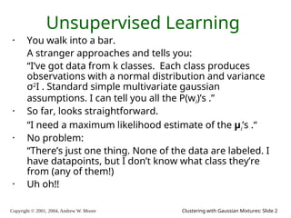
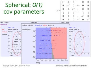
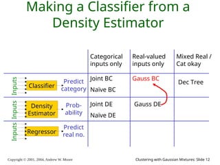
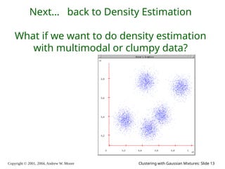
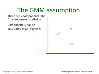
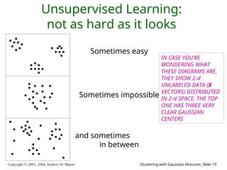
The document is a lecture slide set by Andrew W. Moore discussing clustering with Gaussian mixtures in the context of unsupervised learning. It introduces concepts like maximum likelihood estimation of class means and the Expectation-Maximization (EM) algorithm for density estimation. The slides illustrate various Gaussian mixture models and their applications in estimating parameters from unlabeled data.

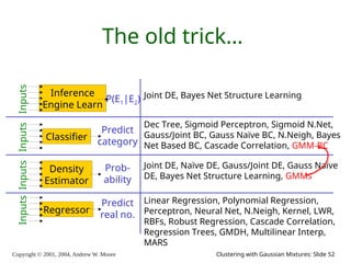
![Copyright © 2001, 2004, Andrew W. Moore Clustering with Gaussian Mixtures: Slide 21
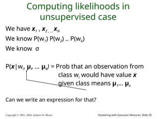
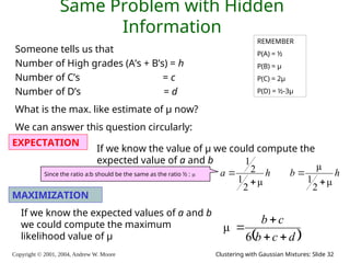
likelihoods in unsupervised
case
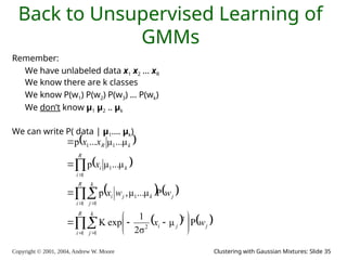
We have x1 x2 … xn
We have P(w1) .. P(wk). We have σ.
We can define, for any x , P(x|wi , μ1, μ2 .. μk)
Can we define P(x | μ1, μ2 .. μk) ?
Can we define P(x1, x1, .. xn | μ1, μ2 .. μk) ?
[YES, IF WE ASSUME THE X1’S WERE DRAWN INDEPENDENTLY]](https://image.slidesharecdn.com/gmm-241104072129-c4bc012f/85/gmatrix-distro_gmatrix-distro_gmatrix-distro-21-320.jpg)
![Copyright © 2001, 2004, Andrew W. Moore Clustering with Gaussian Mixtures: Slide 34
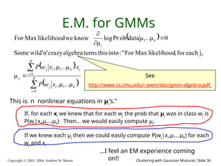
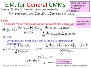
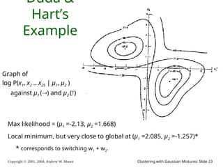
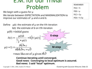
E.M. Convergence
• Convergence proof based on fact that Prob(data | μ) must increase
or remain same between each iteration [NOT OBVIOUS]
• But it can never exceed 1 [OBVIOUS]
So it must therefore converge [OBVIOUS]
t μ(t) b(t)
0 0 0
1 0.0833 2.857
2 0.0937 3.158
3 0.0947 3.185
4 0.0948 3.187
5 0.0948 3.187
6 0.0948 3.187
In our example,
suppose we had
h = 20
c = 10
d = 10
μ(0) = 0
Convergence is generally linear: error
decreases by a constant factor each time
step.](https://image.slidesharecdn.com/gmm-241104072129-c4bc012f/85/gmatrix-distro_gmatrix-distro_gmatrix-distro-34-320.jpg)