Topic 7 Basic Ray Tracing Algorithms and ray tracing.ppt

Topic 7 Ray Tracing
Dr. Collins Oduor
Kenyatta University

 A general mechanism for sampling paths of light in a 3D
scene
 • We will use this mechanism in path tracing
 • Ray Casting mechanism: – Rays are cast from a point in
space towards a specified direction – Rays are
intersected with geometry primitives – The closest
intersection is regarded as a ray “hit” – Lighting or other
attributes are evaluated at the hit location
2

3
Objectives
 Develop a basic recursive ray tracer
 Computer intersections for quadrics and polygons
Angel and Shreiner:
Interactive Computer
Graphics 7E © Addison-
Wesley 2015

Who Determines What Rays to Spawn?
 • Material properties:
 – Reflectance
 – Incandescence
 – Gloss – Permeability a
 – Index of refraction n – …
 • Number, size and type of lights
4

Ray Data Structures
 – Requirements
 • Degradation effects (absorption, scattering, splitting):
– “strength” indicator (opposite of attenuation) –
Optionally, recursion depth
 • Distance sorting of hit points: – Avoid keeping all
intersections and post-sort results – Keep nearest
intersection point or – Cache distance to nearest hit
point
 • Local properties of hit point: – Need to keep track of
hit material, primitive and local attributes (e.g. normal)
A Ray as a Data Struct
5

6
Ray Tracing
 Follow rays of light from a point source
 Can account for reflection and transmission
Angel and Shreiner:
Wesley 2015

7
Computation
 Should be able to handle all physical interactions
 Ray tracing paradigm is not computational
 Most rays do not affect what we see
 Scattering produces many (infinite) additional rays
 Alternative: ray casting
Angel and Shreiner:
Wesley 2015

Stages of raytracing
 • Setting the camera and the image plane
 • Computing a ray from the eye to every pixel and trace
it in the scene
 • Object-ray intersections
 • Shadow, reflected and refracted ray at Shadow,
reflected and refracted ray at each intersection
8

9
surface in a very specific direction (and therefore not a
random one) defined by the geometry's topology and the
photon incoming direction at the point of intersection. The
surface of a diffuse object appears smooth if we look at it with
our eyes. Although if we look at it with a microscope, we
realize that the micro-structure is very complex and not
smooth at all. The image on the left is a photograph of paper
with different magnification scales. Photons are so small that
they are reflected by the micro-features and shapes on the
object's surface. If a beam of light hits the surface of this
diffuse object, photons contained within the volume of the
beam will hit very different parts of the micro-structure and,
therefore, will be reflected in lots of different directions. So
many, that we say, "every possible direction". If we want to
simulate this interaction between the photons and the micro-
structure, we shoot rays in random directions, which,
statistically speaking, is about the same as if they were
reflected in every possible direction.
Sometimes the structure of the material at the macro level is
organized in patterns which can cause the surface of an object
to reflect light in particular directions. This is described as an
anisotropic reflection and will be explained in details in the
lesson on light-materials interaction. The macro structure of
the material can also be the cause of unusual visual effects
such as irridescence which we can observe of butterflies wings
for instance.
We can now begin to look at the situation in terms of computer graphics.
First, we replace our eyes with an image plane composed of pixels. In this
case, the photons emitted will hit one of the many pixels on the image
plane, increasing the brightness at that point to a value greater than zero.
This process is repeated multiple times until all the pixels are adjusted,
creating a computer generated image. This technique is called forward
ray-tracing because we follow the path of the photon forward from the
light source to the observer.
However do you see a potential problem with this approach?
The problem is the following: in our example we assumed that the
reflected photon always intersected the surface of the eye. In reality, rays
are essentially reflected in every possible direction, each of which have a
very, very small probability of actually hitting the eye. We would potentially

10
Ray Casting
 Only rays that reach the eye matter
 Reverse direction and cast rays
 Need at least one ray per pixel
Angel and Shreiner:
Wesley 2015

11
Ray Casting Quadrics
 Ray casting has become the standard way to visualize
quadrics which are implicit surfaces in CSG systems
 Constructive Solid Geometry
 Primitives are solids
 Build objects with set operations
 Union, intersection, set difference
Angel and Shreiner:
Wesley 2015

12
Ray Casting a Sphere
 Ray is parametric
 Sphere is quadric
 Resulting equation is a scalar quadratic equation which
gives entry and exit points of ray (or no solution if ray
misses)
Angel and Shreiner:
Wesley 2015

13
Shadow Rays
 Even if a point is visible, it will not be lit unless we can
see a light source from that point
 Cast shadow or feeler rays
Angel and Shreiner:
Wesley 2015

14
Reflection
 Must follow shadow rays off reflecting or transmitting
surfaces
 Process is recursive
Angel and Shreiner:
Wesley 2015

15
Reflection and Transmission
Angel and Shreiner:
Wesley 2015

16
Diffuse Surfaces
 Theoretically the scattering at each point of intersection
generates an infinite number of new rays that should be
traced
 In practice, we only trace the transmitted and reflected
rays but use the modified Phong model to compute
shade at point of intersection
 Radiosity works best for perfectly diffuse (Lambertian)
surfaces
Angel and Shreiner:
Wesley 2015

17
Building a Ray Tracer
 Best expressed recursively
 Can remove recursion later
 Image based approach
 For each ray …….
 Find intersection with closest surface
 Need whole object database available
 Complexity of calculation limits object types
 Compute lighting at surface
 Trace reflected and transmitted rays
Angel and Shreiner:
Wesley 2015

18
When to stop
 Some light will be absorbed at each intersection
 Track amount left
 Ignore rays that go off to infinity
 Put large sphere around problem
 Count steps
Angel and Shreiner:
Wesley 2015

19
Recursive Ray Tracer
color c = trace(point p, vector d, int step)
{
color local, reflected,
transmitted;
point q;
normal n;
if(step > max)
return(background_color);
Angel and Shreiner:
Wesley 2015

20
q = intersect(p, d, status);
if(status==light_source)
return(light_source_color);
if(status==no_intersection)
return(background_color);
n = normal(q);
r = reflect(q, n);
t = transmit(q,n);
Angel and Shreiner:
Wesley 2015

21
local = phong(q, n, r);
reflected = trace(q, r, step+1);
transmitted = trace(q,t, step+1);
return(local+reflected+
transmitted);
Angel and Shreiner:
Wesley 2015

22
Computing Intersections
 Implicit Objects
 Quadrics
 Planes
 Polyhedra
 Parametric Surfaces
Angel and Shreiner:
Wesley 2015

23
Polyhedra
 Generally we want to intersect with closed convex
objects such as polygons and polyhedra rather than
planes
 Hence we have to worry about inside/outside testing
 For convex objects such as polyhedra there are some
fast tests
Angel and Shreiner:
Wesley 2015

24
Ray Tracing Polyhedra
 If ray enters an object, it must enter a front facing
polygon and leave a back facing polygon
 Polyhedron is formed by intersection of planes
 Ray enters at furthest intersection with front
facing planes
 Ray leaves at closest intersection with back facing
planes
 If entry is further away than exit, ray must miss
the polyhedron
Angel and Shreiner:
Wesley 2015

Advanced Graphics
Lecture Three
Illumination:
Ray tracing effects
and global lighting
Benton,
University
of
Cambridge
–
A.Benton@damtp.cam.ac.uk
orted
in
part
by
Google
UK,
Ltd
Cover
image:
“Cornell
Box”
by
Steven
Parker,
University
of
Utah.
A
tera-ray
monte-carlo
rendering
of
the
Cornell
Box,
generated
in
2
CPU
years
on
an
Origin
2000.
The
full
image
contains
2048
x
2048
pixels
with
over
100,000
primary
rays
per
pixel
(317
x
317
jittered
samples).
Over
one
trillion
rays
were
traced
in
the
generation
of
this
image.

Lighting revisited
 We approximate lighting as the sum of the ambient,
diffuse, and specular components of the light reflected to
the eye.
 Associate scalar parameters
kA, kD and kS with the surface.
 Calculate diffuse and specular
from each light source separately.
O
N
D
P
R
L1
L2

Lighting revisited—ambient lighting
 Ambient light is a flat scalar constant, LA.
 The amount of ambient light LA is a parameter of the
scene; the way it illuminates a particular surface is a
parameter of the surface.
 Some surfaces (ex: cotton wool) have high ambient
coefficient kA; others (ex: steel tabletop) have low kA.
 Lighting intensity for ambient light alone:
A
A
A L
k
P
I 
)
(

Lighting revisited—diffuse lighting
 The diffuse coefficient kD measures how much light
scatters off the surface.
 Some surfaces (e.g. skin) have high kD, scattering light from
many microscopic facets and breaks. Others (e.g. ball
bearings) have low kD.
 Diffuse lighting intensity:
)
(
)
(cos
)
(
L
N
L
k
L
k
P
I
D
D
D
D
D


 
N N
θ
L
L

Lighting revisited—specular lighting
 The specular coefficient kS measures how much light
reflects off the surface.
 A ball bearing has high kS; I don’t.
 ‘Shininess’ is approximated by a scalar power n.
 Specular lighting intensity:
n
S
S
n
S
S
n
S
S
S
E
L
k
E
R
L
k
L
k
P
I
)
•
L)
N)N
•
2(L
((
)
•
(
)
(cos
)
(



  N
α L
R
E

Ambient=1
Diffuse=0
Specular=0
Ambient=0
Diffuse=1
Specular=0
Ambient=0.2
Diffuse=0.4
Specular=0.4
(n
=2)
Ambient=0
Diffuse=0
Specular=1
(n
=2)

Spotlights
 To create a spotlight shining along axis S, you can
multiply the (diffuse+specular) term by (max(L•S,0))m
.
 Raising m will tighten the spotlight,
but leave the edges soft.
 If you’d prefer a hard-edged spotlight
of uniform internal intensity, you can
use a conditional, e.g.
((L•S > cos(15˚)) ? 1 : 0).
O
D
P
θ
L
S

 To simulate shadow in ray tracing, fire a ray from P
towards each light Li. If the ray hits another object
before the light, then discard Li in the sum.
 This is a boolean removal, so it
will give hard-edged shadows.
 Hard-edged shadows imply a
pinpoint light source.
Ray tracing—Shadows

Softer shadows
 Shadows in nature are not sharp because light sources are
not infinitely small.
 Also because light scatters, etc.
 For lights with volume, fire many rays, covering the cross-
section of your illuminated space.
 Illumination is (the total number of rays
that aren’t blocked) divided by (the total
number of rays fired).
 This is an example of Monte-Carlo integration:
a coarse simulation of an integral over a space
by randomly sampling it with many rays.
 The more rays fired, the smoother the result.
O
D
P
L1

Reflection
 Reflection rays are calculated by:
R = 2(-D•N)N+D
…just like the specular reflection ray.
 Finding the reflected color is a
recursive raycast.
 Reflection has scene-dependant
performance impact.
O
D
P
L1
Q

num bounces=1
num bounces=0 num bounces=2
num bounces=3

Transparency
 To add transparency, generate and trace a new
transparency ray with OT=P, DT=D.
 Option 1 (object state):
 Associate a transparency value A with the
material of the surface, like reflection.
 Option 2 (RGBA):
 Make color a 1x4 vector where the fourth
component, ‘alpha’, determines the weight
of the recursed transparency ray.

Refraction
 The angle of incidence of a ray of light where it strikes a
surface is the acute angle between the ray and the
surface normal.
 The refractive index of a material is a measure of how
much the speed of light1
is reduced inside the material.
 The refractive index of air is about 1.003.
 The refractive index of water is about 1.33.
1
Or sound waves or other waves

What’s wrong with raytracing?
 Soft shadows are expensive
 Shadows of transparent objects
require further coding or hacks
 Lighting off reflective objects follows
different shadow rules from normal
lighting
 Hard to implement diffuse reflection
(color bleeding, such as in the
Cornell Box—notice how the sides of
the inner cubes are shaded red and
green.)
 Fundamentally, the ambient term is
a hack and the diffuse term is only
one step in what should be a
recursive, self-reinforcing series.
The Cornell Box is a test for rendering
Software, developed at Cornell University
in 1984 by Don Greenberg. An actual
box is built and photographed; an identical
scene is then rendered in software and the
two images are compared.

Radiosity
 Radiosity is an illumination method
which simulates the global
dispersion and reflection of diffuse
light.
 First developed for describing
spectral heat transfer (1950s)
 Adapted to graphics in the 1980s at
Cornell University
 Radiosity is a finite-element
approach to global illumination: it
breaks the scene into many small
elements (‘patches’) and calculates
the energy transfer between them.
Images from Cornell University’s graphics group
http://www.graphics.cornell.edu/online/research/

Radiosity—algorithm
 Surfaces in the scene are divided into form factors (also
called patches), small subsections of each polygon or object.
 For every pair of form factors A, B, compute a view factor
describing how much energy from patch A reaches patch B.
 The further apart two patches are in space or orientation, the
less light they shed on each other, giving lower view factors.
 Calculate the lighting of all directly-lit patches.
 Bounce the light from all lit patches to all those they light,
carrying more light to patches with higher relative view
factors. Repeating this step will distribute the total light
across the scene, producing a total illumination model.
Note: very unfortunately, some literature
uses the term ‘form factor’ for the view
factor as well.

Radiosity—mathematical support
 The ‘radiosity’ of a single patch is the amount of energy
leaving the patch per discrete time interval.
 This energy is the total light being emitted directly from the
patch combined with the total light being reflected by the
patch:
where…

Bi is the radiosity of patch i;
Bj is the cumulative radiosity of all other patches (j≠i)

Ei is the emitted energy of the patch

Ri is the reflectivity of the patch

Fij is the view factor of energy from patch i to patch j.




n
j
ij
j
i
i
i F
B
R
E
B
1

Radiosity—form factors
 Finding form factors can be done
procedurally or dynamically
 Can subdivide every surface into small
patches of similar size
 Can dynamically subdivide wherever the
1st
derivative of calculated intensity rises
above some threshold.
 Computing cost for a general radiosity
solution goes up as the square of the
number of patches, so try to keep
patches down.
 Subdividing a large flat white wall could
be a waste.
 Patches should ideally closely align
with lines of shadow.

Radiosity—implementation
(A) Simple patch triangulation
(B) Adaptive patch generation: the floor
and walls of the room are dynamically
subdivided to produce more patches
where shadow detail is higher.
Images from “Automatic
generation of node spacing
function”, IBM (1998)
http://www.trl.ibm.com/
projects/meshing/nsp/nspE.htm
(A) (B)

Radiosity—view factors
 One equation for the view factor
between patches i, j is:
…where θi is the angle between the
normal of patch i and the line to
patch j, r is the distance and V(i,j) is
the visibility from i to j (0 for
occluded, 1 for clear line of sight.)
High view factor
Low view factor
θi
θj
)
,
(
cos
cos
2
j
i
V
r
j
Fi
j
i






Radiosity—calculating visibility
 Calculating V(i,j) can be slow.
 One method is the hemicube, in which each form factor is
encased in a half-cube. The scene is then ‘rendered’ from the
point of view of the patch, through the walls of the
hemicube; V(i,j) is computed for each patch based on which
patches it can see (and at what percentage) in its hemicube.
 A purer method, but more computationally expensive, uses
hemispheres.
Note: This method can be
accelerated using modern
graphics hardware to render
the scene.
The scene is ‘rendered’ with
flat lighting, setting the ‘color’
of each object to be a pointer
to the object in memory.

Radiosity gallery
Teapot (wikipedia)
Image from
GPU Gems II, nVidia
Image from A Two Pass Solution to the Rendering Equation:
a Synthesis of Ray Tracing and Radiosity Methods,
John R. Wallace, Michael F. Cohen and Donald P. Greenberg
(Cornell University, 1987)

Shadows, refraction and caustics
 Problem: shadow ray strikes
transparent, refractive
object.
 Refracted shadow ray will
now miss the light.
 This destroys the validity of
the boolean shadow test.
 Problem: light passing
through a refractive object
will sometimes form caustics
(right), artifacts where the
envelope of a collection of
rays falling on the surface is
bright enough to be visible. This is a photo of a real pepper-shaker.
Note the caustics to the left of the shaker, in and
outside of its shadow.
Photo credit: Jan Zankowski

Shadows, refraction and caustics
 Solutions for shadows of transparent objects:
 Backwards ray tracing (Arvo)
 Very computationally heavy
 Improved by stencil mapping (Shenya et al)
 Shadow attenuation (Pierce)
 Low refraction, no caustics
 More general solution:
 Photon mapping (Jensen)→
Image from http://graphics.ucsd.edu/~henrik/
Generated with photon mapping

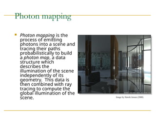
Photon mapping
 Photon mapping is the
process of emitting
photons into a scene and
tracing their paths
probabilistically to build
a photon map, a data
structure which
describes the
illumination of the scene
independently of its
geometry. This data is
then combined with ray
tracing to compute the
global illumination of the
scene. Image by Henrik Jensen (2000)

Photon mapping—algorithm (1/2)
Photon mapping is a two-pass algorithm:
1. Photon scattering
1. Photons are fired from each light source, scattered in
randomly-chosen directions. The number of photons
per light is a function of its surface area and brightness.
2. Photons fire through the scene (re-use that raytracer,
folks.) Where they strike a surface they are either
absorbed, reflected or refracted.
3. Wherever energy is absorbed, cache the location,
direction and energy of the photon in the photon map.
The photon map data structure must support fast
insertion and fast nearest-neighbor lookup; a kd-tree1
is
often used.
1
A kd-tree is a type of binary space partitioning tree. Space is recursively
subdivided by axis-aligned planes and points on either side of each plane
are separated in the tree. The kd-tree has O(n log n) insertion time (but
this is very optimizable by domain knowledge) and O(n2/3
) search time.
Image by Zack Waters

Photon mapping—algorithm (2/2)
Photon mapping is a two-pass algorithm:
2. Rendering
1. Ray trace the scene from the point of view of the
camera.
2. For each first contact point P use the ray tracer for
specular but compute diffuse from the photon map and
do away with ambient completely.
3. Compute radiant illumination by summing the
contribution along the eye ray of all photons within a
sphere of radius r of P.
4. Caustics can be calculated directly here from the photon
map. For speed, the caustic map is usually distinct from
the radiance map.
Image by Zack Waters

Photon mapping—a few comments
 This method is a great
example of Monte Carlo
integration, in which a difficult
integral (the lighting equation)
is simulated by randomly
sampling values from within
the integral’s domain until
enough samples average out
to about the right answer.
 This means that you’re going
to be firing millions of photons.
Your data structure is going to
have to be very space-efficient.
http://www.okino.com/conv/imp_jt.htm

Photon mapping—a few comments
 Initial photon direction is random. Constrained
by light shape, but random.
 What exactly happens each time a photon hits a
solid also has a random component:
 Based on the diffuse reflectance, specular reflectance and
transparency of the surface, compute probabilities pd, ps
and pt where (pd+ps+pt) 1. This gives a probability map:
≤
 Choose a random value p є [0,1]. Where p falls in the
probability map of the surface determines whether the
photon is reflected, refracted or absorbed.
0 1
pd ps pt
This surface would
have minimal
specular highlight.

Photon mapping gallery
http://www.pbrt.org/gallery.php
http://web.cs.wpi.edu/~emmanuel/courses/cs563/
write_ups/zackw/photon_mapping/
PhotonMapping.html
http://graphics.ucsd.edu/~henrik/images/global.html

References
Ray tracing|
 Foley & van Dam, Computer Graphics (1995)
 Jon Genetti and Dan Gordon, Ray Tracing With Adaptive Supersampling in Object Space,
http://www.cs.uaf.edu/~genetti/Research/Papers/GI93/GI.html (1993)
 Zack Waters, “Realistic Raytracing”,
http://web.cs.wpi.edu/~emmanuel/courses/cs563/write_ups/zackw/realistic_raytraci
ng.html
Radiosity
 nVidia: http://http.developer.nvidia.com/GPUGems2/gpugems2_chapter39.html
 Cornell: http://www.graphics.cornell.edu/online/research/
 Wallace, J. R., K. A. Elmquist, and E. A. Haines. 1989, “A Ray Tracing Algorithm for
Progressive Radiosity.” In Computer Graphics (Proceedings of SIGGRAPH 89) 23(4), pp.
315–324.
 Buss, “3-D Computer Graphics: A Mathematical Introduction with OpenGL” (Chapter
XI), Cambridge University Press (2003)
Photon mapping
 Henrik Jenson, “Global Illumination using Photon Maps”,
http://graphics.ucsd.edu/~henrik/
 Zack Waters, “Photon Mapping”,
http://web.cs.wpi.edu/~emmanuel/courses/cs563/write_ups/zackw/photon_mapping
/PhotonMapping.html

Topic 7 Basic Ray Tracing Algorithms and ray tracing.ppt

More Related Content

Similar to Topic 7 Basic Ray Tracing Algorithms and ray tracing.ppt

Recently uploaded

Topic 7 Basic Ray Tracing Algorithms and ray tracing.ppt