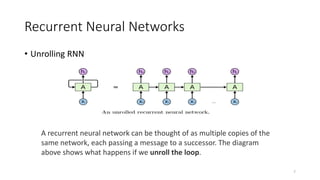
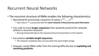
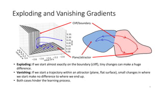
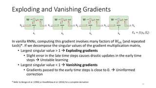
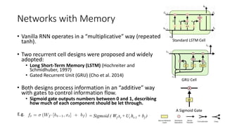
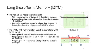
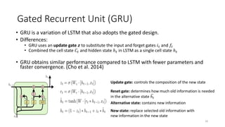
The document provides an overview of recurrent neural networks (RNNs), including their implementation and applications. It discusses how RNNs can process sequential data due to their ability to preserve information from previous time steps. However, vanilla RNNs suffer from exploding and vanishing gradients during training. Newer RNN architectures like LSTMs and GRUs address this issue through gated connections that allow for better propagation of errors. Sequence learning tasks that can be addressed with RNNs include time-series forecasting, language processing, and image/video caption generation. The document outlines RNN architectures for different types of sequential inputs and outputs.

1. An Introduction to
Recurrent Neural Networks:
Overview, Implementation, and Application
Hongyi Zhu and Hsinchun Chen
Artificial Intelligence Lab, University of Arizona
Updated April 2020
1

2. Acknowledgements
• Selected pictures and Ccontents from: Andrew Ng, Stanford
University, Chris Olah, Google Brain, Fei-Fei Li, Stanford University,
Geoffrey Hinton, Google & University of Toronto, Hung-yi Lee,
National Taiwan University, Ian Goodfellow, Google Brain, Yann LeCun,
New York University, Yoshua Bengio, Universite de Montreal
• Colah’s Blog, “Understanding LSTM Networks,” 2015
• I. Witten, et al., “Data Mining,” 2017
2

3. Outline
• Recurrent Neural Networks
• Vanilla RNN
• Exploding and Vanishing Gradients
• Networks with Memory
• Long Short-Term Memory (LSTM)
• Gated Recurrent Unit (GRU)
• Sequence Learning Architectures
• Sequence Learning with one RNN Layer
• Sequence Learning with multiple RNN Layers
• Implementation example using Keras in Python: sentiment analysis
• Application: Sequence-to-Sequence Model in Activities of Daily Living (ADL)
Recognition
3

4. Recurrent Neural Networks
• Human brain deals with information streams. Most data is obtained, processed, and
generated sequentially.
• E.g., listening: soundwaves  vocabularies/sentences
• E.g., action: brain signals/instructions  sequential muscle movements
• Human thoughts have persistence; humans don’t start their thinking from scratch
every second.
• As you read this sentence, you understand each word based on your prior knowledge.
• The applications of standard Artificial Neural Networks (and also Convolutional
Networks) are limited due to:
• They only accepted a fixed-size vector as input (e.g., an image) and produce a fixed-size vector
as output (e.g., probabilities of different classes).
• These models use a fixed amount of computational steps (e.g. the number of layers in the
model).
• Recurrent Neural Networks (RNNs) are a family of neural networks introduced to
learn sequential data.
• Inspired by the temporal-dependent and persistent human thoughts
4

5. Real-life Sequence Learning Applications
• RNNs can be applied to various type of sequential data to learn the
temporal patterns.
• Time-series data (e.g., stock price)  Prediction, regression
• Raw sensor data (e.g., signal, voice, handwriting)  Labels or text sequences
• Text  Label (e.g., sentiment) or text sequence (e.g., translation, summary, answer)
• Image and video  Text description (e.g., captions, scene interpretation)
5
Task Input Output
Activity Recognition (Zhu et al. 2018) Sensor Signals Activity Labels
Machine translation (Sutskever et al. 2014) English text French text
Question answering (Bordes et al. 2014) Question Answer
Speech recognition (Graves et al. 2013) Voice Text
Handwriting prediction (Graves 2013) Handwriting Text
Opinion mining (Irsoy et al. 2014) Text Opinion expression

6. Recurrent Neural Networks
• Recurrent Neural Networks are networks with loops,
allowing information to persist.
6
In the above diagram, a chunk of neural
network, A = fW, looks at some
input xt and outputs a value ht. A loop
allows information to be passed from
one step of the network to the next.
Output is to predict a vector ht,
where 𝑜𝑢𝑡𝑝𝑢𝑡 𝑦𝑡 = 𝜑(ℎ𝑡) at some
time steps (t)

7. Recurrent Neural Networks
• Unrolling RNN
7
A recurrent neural network can be thought of as multiple copies of the
same network, each passing a message to a successor. The diagram
above shows what happens if we unroll the loop.

8. Recurrent Neural Networks
• The recurrent structure of RNNs enables the following characteristics:
• Specialized for processing a sequence of values 𝑥 1 , … , 𝑥 𝜏
• Each value 𝑥 𝑖 is processed with the same network A that preserves past information
• Can scale to much longer sequences than would be practical for networks
without a recurrent structure
• Reusing network A reduces the required amount of parameters in the network
• Can process variable-length sequences
• The network complexity does not vary when the input length change
• However, vanilla RNNs suffer from the training difficulty due to exploding and
vanishing gradients.
8

9. Exploding and Vanishing Gradients
• Exploding: If we start almost exactly on the boundary (cliff), tiny changes can make a huge
difference.
• Vanishing: If we start a trajectory within an attractor (plane, flat surface), small changes in where
we start make no difference to where we end up.
• Both cases hinder the learning process.
9
Cliff/boundary
Plane/attractor

10. Exploding and Vanishing Gradients
In vanilla RNNs, computing this gradient involves many factors of 𝑊ℎℎ (and repeated
tanh)*. If we decompose the singular values of the gradient multiplication matrix,
• Largest singular value > 1  Exploding gradients
• Slight error in the late time steps causes drastic updates in the early time
steps  Unstable learning
• Largest singular value < 1  Vanishing gradients
• Gradients passed to the early time steps is close to 0.  Uninformed
correction
10
* Refer to Bengio et al. (1994) or Goodfellow et al. (2016) for a complete derivation
𝐸4 = 𝐽(𝑦4, 𝑦4)

11. Networks with Memory
• Vanilla RNN operates in a “multiplicative” way (repeated
tanh).
• Two recurrent cell designs were proposed and widely
adopted:
• Long Short-Term Memory (LSTM) (Hochreiter and
Schmidhuber, 1997)
• Gated Recurrent Unit (GRU) (Cho et al. 2014)
• Both designs process information in an “additive” way
with gates to control information flow.
• Sigmoid gate outputs numbers between 0 and 1, describing
how much of each component should be let through.
11
Standard LSTM Cell
GRU Cell
A Sigmoid Gate
= Sigmoid ( Wf xt + Ut ht-1 + bf )
E.g.

12. Long Short-Term Memory (LSTM)
• The key to LSTMs is the cell state.
• Stores information of the past  long-term memory
• Passes along time steps with minor linear interactions
 “additive”
• Results in an uninterrupted gradient flow  errors in
the past pertain and impact learning in the future
• The LSTM cell manipulates input information with
three gates.
• Input gate  controls the intake of new information
• Forget gate  determines what part of the cell state to
be updated
• Output gate  determines what part of the cell state
to output
12
Gradient Flow
Cell State 𝐶𝑡

13. 13
LSTM: Components & Flow
• LSM unit output
• Output gate units
• Transformed memory cell contents
• Gated update to memory cell units
• Forget gate units
• Input gate units
• Potential input to memory cell

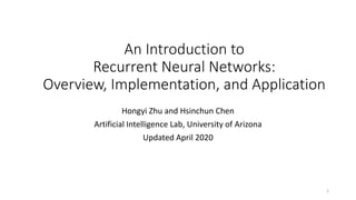
14. Step-by-step LSTM Walk Through
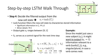
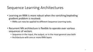
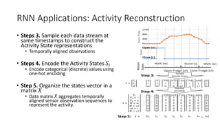
• Step 1: Decide what information to throw away from the cell state
(memory) 
• The output of the previous state ℎ𝑡−1 and the new information 𝑥𝑡 jointly
determine what to forget
• ℎ𝑡−1 contains selected features from the memory 𝐶𝑡−1
• Forget gate 𝑓𝑡 ranges between [0, 1]
14
Forget gate
Text processing example:
Cell state may include the gender
of the current subject (ℎ𝑡−1).
When the model observes a new
subject (𝑥𝑡), it may want to forget
(𝑓𝑡 → 0) the old subject in the
memory (𝐶𝑡−1).

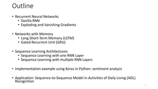
15. Step-by-step LSTM Walk Through
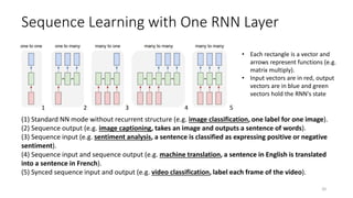
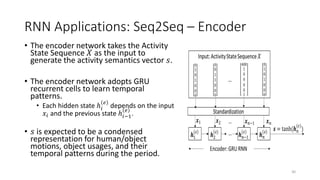
• Step 2: Prepare the updates for the cell state
from input 
• An alternative cell state 𝐶𝑡 is created from the new information 𝑥𝑡 with the
guidance of ℎ𝑡−1.
• Input gate 𝑖𝑡 ranges between [0, 1]
15
Input gate Alternative
cell state
Example:
The model may want to add
(𝑖𝑡 → 1) the gender of new
subject (𝐶𝑡) to the cell state to
replace the old one it is
forgetting.

16. Step-by-step LSTM Walk Through
• Step 3: Update the cell state 
• The new cell state 𝐶𝑡 is comprised of information from the past 𝑓𝑡 ∗ 𝐶𝑡−1 and
valuable new information 𝑖𝑡 ∗ 𝐶𝑡
• ∗ denotes elementwise multiplication
16
New cell state
Example:
The model drops the old gender
information (𝑓𝑡 ∗ 𝐶𝑡−1) and adds
new gender information (𝑖𝑡 ∗ 𝐶𝑡) to
form the new cell state (𝐶𝑡).

17. Step-by-step LSTM Walk Through
• Step 4: Decide the filtered output from the
new cell state 
• tanh function filters the new cell state to characterize stored information
• Significant information in 𝐶𝑡  ±1
• Minor details  0
• Output gate 𝑜𝑡 ranges between 0, 1
• ℎ𝑡 serves as a control signal for the next time step
17
Output gate
Example:
Since the model just saw a
new subject (𝑥𝑡), it might
want to output (𝑜𝑡 → 1)
information relevant to a
verb (tanh(𝐶𝑡)), e.g.,
singular/plural, in case a
verb comes next.

18. Gated Recurrent Unit (GRU)
• GRU is a variation of LSTM that also adopts the gated design.
• Differences:
• GRU uses an update gate 𝒛 to substitute the input and forget gates 𝑖𝑡 and 𝑓𝑡
• Combined the cell state 𝐶𝑡 and hidden state ℎ𝑡 in LSTM as a single cell state ℎ𝑡
• GRU obtains similar performance compared to LSTM with fewer parameters and
faster convergence. (Cho et al. 2014)
18
Update gate: controls the composition of the new state
Reset gate: determines how much old information is needed
in the alternative state ℎ𝑡
Alternative state: contains new information
New state: replace selected old information with
new information in the new state

19. Sequence Learning Architectures
• Learning on RNN is more robust when the vanishing/exploding
gradient problem is resolved.
• RNNs can now be applied to different Sequence Learning tasks.
• Recurrent NN architecture is flexible to operate over various
sequences of vectors.
• Sequence in the input, the output, or in the most general case both
• Architecture with one or more RNN layers
19

20. Sequence Learning with One RNN Layer
20
• Each rectangle is a vector and
arrows represent functions (e.g.
matrix multiply).
• Input vectors are in red, output
vectors are in blue and green
vectors hold the RNN's state
(1) Standard NN mode without recurrent structure (e.g. image classification, one label for one image).
(2) Sequence output (e.g. image captioning, takes an image and outputs a sentence of words).
(3) Sequence input (e.g. sentiment analysis, a sentence is classified as expressing positive or negative
sentiment).
(4) Sequence input and sequence output (e.g. machine translation, a sentence in English is translated
into a sentence in French).
(5) Synced sequence input and output (e.g. video classification, label each frame of the video).
1 2 3 4 5

21. Sequence Learning with Multiple RNN Layers
• Bidirectional RNN
• Connects two recurrent units (synced
many-to-many model) of opposite
directions to the same output.
• Captures forward and backward
information from the input sequence
• Apply to data whose current state (e.g.,
ℎ0) can be better determined when given
future information (e.g., 𝑥1, 𝑥2, … , 𝑥𝑡)
• E.g., in the sentence “the bank is robbed,” the
semantics of “bank” can be determined given
the verb “robbed.”
21
B
B
B
B

22. Sequence Learning with Multiple RNN Layers
• Sequence-to-Sequence (Seq2Seq) model
• Developed by Google in 2018 for use in machine translation.
• Seq2seq turns one sequence into another sequence. It does so by use of a recurrent
neural network (RNN) or more often LSTM or GRU to avoid the problem of vanishing
gradient.
• The primary components are one Encoder and one Decoder network. The encoder
turns each item into a corresponding hidden vector containing the item and its
context. The decoder reverses the process, turning the vector into an output item,
using the previous output as the input context.
• Encoder RNN: extract and compress the
semantics from the input sequence
• Decoder RNN: generate a sequence based
on the input semantics
• Apply to tasks such as machine
translation
• Similar underlying semantics
• E.g., “I love you.” to “Je t’aime.”
22
B B B B
y0 y1 y2 ym
…
An RNN as the encoder An RNN as the decoder
Input sequence
Encoded semantics
Decoded sequence

23. Implementing RNN in Python using Keras
• Keras provides APIs for the vanilla RNN design, LSTM, and GRU cells:
• keras.layers.SimpleRNN(units, activation='tanh', return_sequences=False, …)
• keras.layers.LSTM(units, activation='tanh', recurrent_activation='hard_sigmoid', …)
• keras.layers.GRU(units, activation='tanh', recurrent_activation='hard_sigmoid', …)
• Critical parameters*
• units: dimensionality of the output space
• activation: activation function to use on the recurrent layer, ‘tanh’ by default
• recurrent_activation: activation function for the gates
• return_sequences:
• True to obtain the output on each time step
• False to obtain the last output
23
*: More can be found on https://keras.io/layers/recurrent/

24. Implementation Example: Sequence Classification with LSTM
• IMDB movie review sentiment classification problem
• Classify each movie review into a sentiment class (positive (1) or negative (0))
24
https://machinelearningmastery.com/sequence-classification-lstm-recurrent-neural-networks-python-keras/
http://ai.stanford.edu/~amaas/data/sentiment/
import numpy
from keras.datasets import imdb // keras provides this built-in dataset
from keras.models import Sequential
from keras.layers import Dense, LSTM
from keras.layers.embeddings import Embedding
from keras.preprocessing import sequence
# fix random seed for reproducibility
numpy.random.seed(7)
# load the dataset but only keep the top n words, zero the rest // data preprocessing
top_words = 5000
(X_train, y_train), (X_test, y_test) = imdb.load_data(num_words=top_words)
# truncate and pad input sequences
max_review_length = 500
X_train = sequence.pad_sequences(X_train, maxlen=max_review_length)
X_test = sequence.pad_sequences(X_test, maxlen=max_review_length)

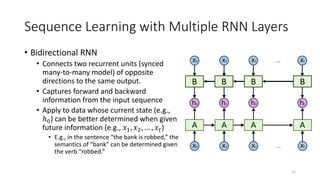
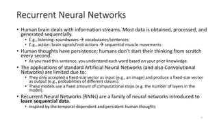
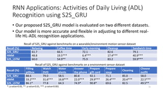
25. Implementation Example: Sequence Classification with LSTM
(many to one)
25
# define word embedding size
embedding_vecor_length = 32
# create a sequential model
model = Sequential()
# transform input sequence into word embedding representation
model.add(Embedding(top_words, embedding_vecor_length,
input_length=max_review_length))
# generate a 100-dimention output, can be replaced by GRU or SimpleRNN
recurrent cells
model.add(LSTM(100))
# a fully connected layer weight the 100-dimention output to one node for
prediction
model.add(Dense(1, activation='sigmoid’))
# use binary_crossentropy as the loss function for the classification
model.compile(loss='binary_crossentropy', optimizer='adam',
metrics=['accuracy'])
print(model.summary())
# model training (for 3 epochs)
model.fit(X_train, y_train, validation_data=(X_test, y_test), epochs=3,
batch_size=64)
# Final evaluation of the model
scores = model.evaluate(X_test, y_test, verbose=0)
print("Accuracy: %.2f%%" % (scores[1]*100))
100 dims
Fully
connected
layer
Word embeddings
Recurrent cell
… movie fantastic, awesome …
Review
32 dims
0/1?

26. RNN Applications: High-level Activities of
Daily Living (HL-ADL) Recognition
• Activities of Daily Living (ADLs) are
introduced to evaluate the self-care
ability of senior citizens (Williams
2014).
• Sensor-based home monitoring
systems
• Environment: Placed in the environment
to capture changes (e.g., on/off, motion)
• Wearable: Attached to the body to
measure movements and physiological
signals
• Sensors sample at 10 Hz  0.8 million
records per day
• Machine learning (esp. deep learning)
needed to recognize ADLs from the
large amount of data
• Mid-level (ML) ADLs: gestures, gait, etc.
• High-level (HL) ADLs: preparing food,
medical intake, senior care, etc.
• Research Objective: develop a
universal ADL recognition framework
to extract HL-ADLs from raw sensor
data
26

27. RNN Applications: Seq2Seq-ADL Research Design
27
• Intuition: Recognizing the HL-ADLs from the sensor data is similar to
captioning/translation. We can generate ADL label sequence with a Seq2Seq
model for the input data. The underlying semantics are similar.
• A Seq2Seq model is designed to extract HL-ADLs from the activity state sequence

28. RNN Applications: Activity Reconstruction
• Objective: create temporally aligned
activity representation from different
data sources
• Four sensors for demonstration:
• a force plate  pressure on the floor
• a door on/off sensor  open (o) and
close (c) states
• a human motion sensor
• object motion sensor attached on the
fridge
• Step 1. Extract discrete motion states
from motion sensor data with a state-
of-the-art gesture recognition model
• Steps 2. Interpolate discrete data from
each sensor
28

29. RNN Applications: Activity Reconstruction
• Steps 3. Sample each data stream at
same timestamps to construct the
Activity State representations
• Temporally aligned observations
• Steps 4. Encode the Activity States 𝑆𝑖
• Encode categorical (discrete) values using
one-hot encoding
• Step 5. Organize the states vector in a
matrix 𝑋
• Data matrix 𝑋 aggregates temporally
aligned sensor observation sequences to
represent the activity.
29

30. RNN Applications: Seq2Seq – Encoder
• The encoder network takes the Activity
State Sequence 𝑋 as the input to
generate the activity semantics vector 𝑠.
• The encoder network adopts GRU
recurrent cells to learn temporal
patterns.
• Each hidden state ℎ𝑖
𝑒
depends on the input
𝑥𝑖 and the previous state ℎ𝑖−1
𝑒
.
• 𝑠 is expected to be a condensed
representation for human/object
motions, object usages, and their
temporal patterns during the period.
30

31. RNN Applications: Seq2Seq – Decoder
• The decoder network takes the encoded
activity semantics vector 𝑠 to generate HL-
ADL label for each input vector.
• The decoder network also adopts GRU
recurrent cells to interpret the temporal
patterns.
• Multi-class classification
• Softmax  probability distribution over output
classes
• Categorical cross-entropy loss
31

32. RNN Applications: Activities of Daily Living (ADL)
Recognition using S2S_GRU
• Our proposed S2S_GRU model is evaluated on two different datasets.
• Our model is more accurate and flexible in adjusting to different real-
life HL-ADL recognition applications.
32
Recall (%)
Filling
pillbox
Watch
DVD
Water
plants
Answer
the phone
Prepare
gift card
Prepare
soup
Cleaning
Choose
outfit
S2S_GRU 88.6 79.0 58.5 80.8 92.1 71.1 85.0 58.0
HMM 33.2*** 31.6*** 16.8*** 22.0*** 29.9*** 26.4*** 20.4*** 22.5***
S2S_LSTM 86.1* 77.8 64.3 74.9* 90.8* 69.6 82.5 49.5**
Recall (%) Relaxing Coffee time Early morning Cleanup Sandwich time
S2S_GRU 61.7 66.5 72.1 82.6 79.1
HMM 48.8 19.5*** 6.4*** 17.4*** 40.9***
S2S_LSTM 60.0 54.9** 75.9 83.2 59.9***
Recall of S2S_GRU against benchmarks on a wearable/environment motion sensor dataset
Recall of S2S_GRU against benchmarks on a environment sensor dataset
*: p-value<0.05, **: p-value<0.01, ***: p-value<0.001

33. Summary
• LSTM and GRU are RNNs that retain past information and update with
a gated design.
• The “additive” structure avoids vanishing gradient problem.
• RNNs allow flexible architecture designs to adapt to different
sequence learning requirements.
• RNNs have broad real-life applications.
• Text processing, machine translation, signal extraction/recognition, image
captioning
• Mobile health analytics, activity of daily living, senior care
33

34. Important References
• Bengio, Y., Simard, P., & Frasconi, P. (1994). Learning long-term dependencies with
gradient descent is difficult. IEEE transactions on neural networks, 5(2), 157-166.
• Goodfellow, I., Bengio, Y., Courville, A., & Bengio, Y. (2016). Deep learning (Vol. 1).
Cambridge: MIT press.
• Graves, A. (2012). Supervised sequence labelling with recurrent neural networks.
https://www.cs.toronto.edu/~graves/preprint.pdf
• Jozefowicz, R., Zaremba, W., & Sutskever, I. (2015, June). An empirical exploration
of recurrent network architectures. In International Conference on Machine
Learning (pp. 2342-2350).
• Lipton, Z. C., Berkowitz, J., & Elkan, C. (2015). A critical review of recurrent neural
networks for sequence learning. arXiv preprint arXiv:1506.00019.
• Salehinejad, H., Baarbe, J., Sankar, S., Barfett, J., Colak, E., & Valaee, S. (2017).
Recent Advances in Recurrent Neural Networks. arXiv preprint arXiv:1801.01078.
34