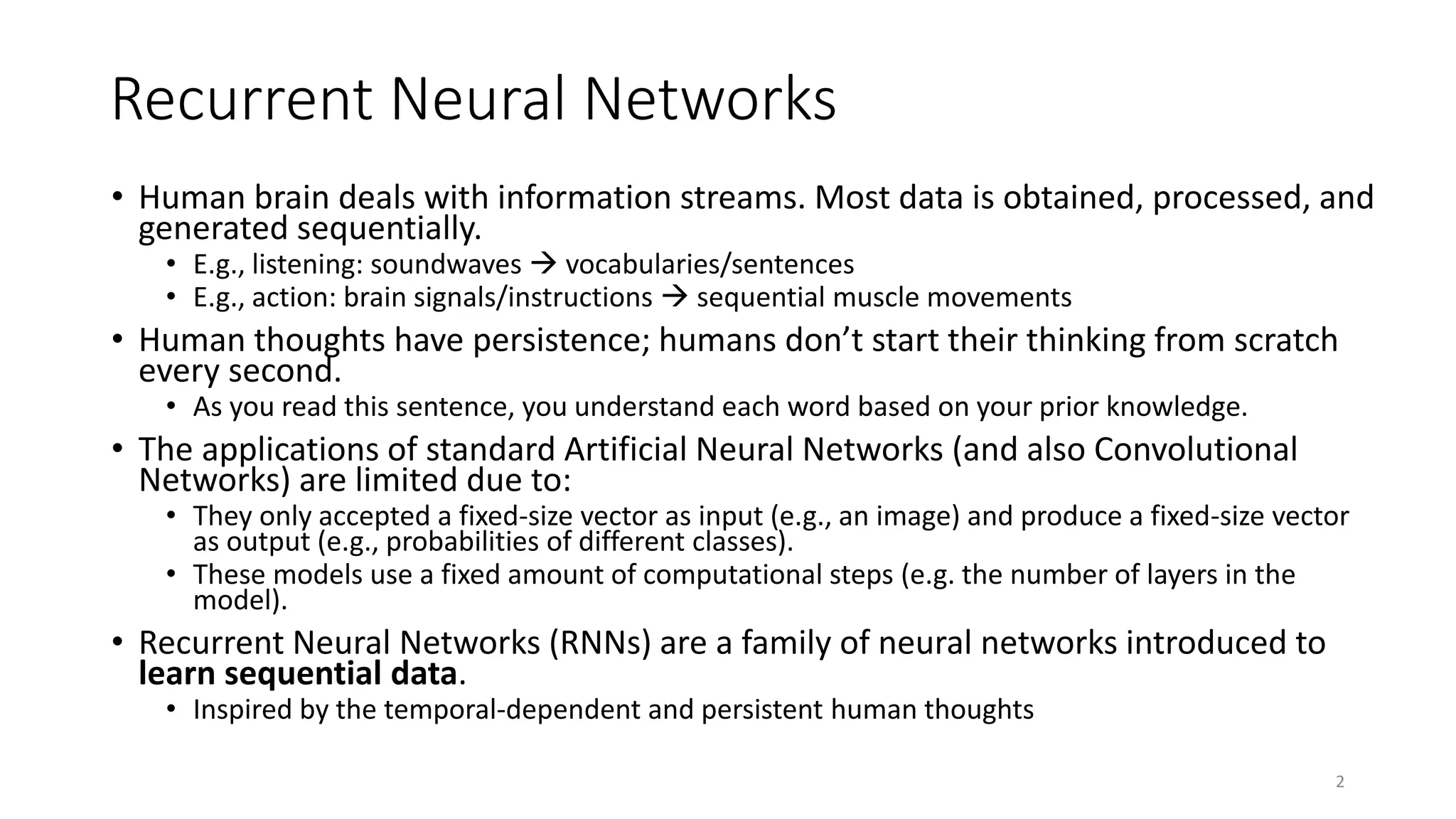
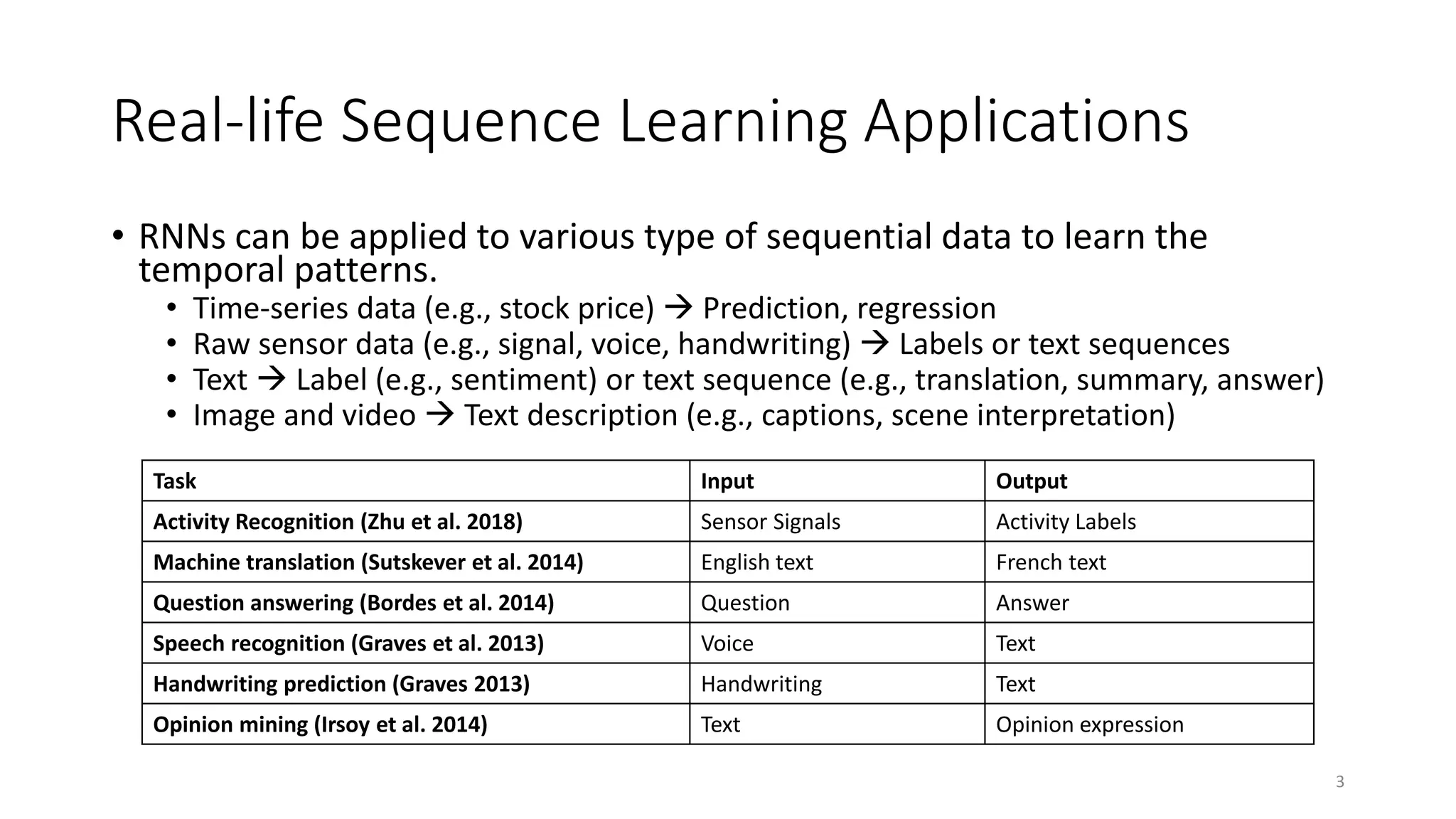
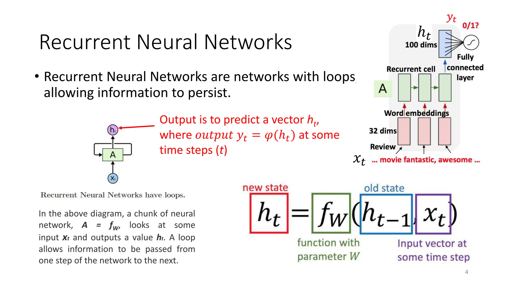
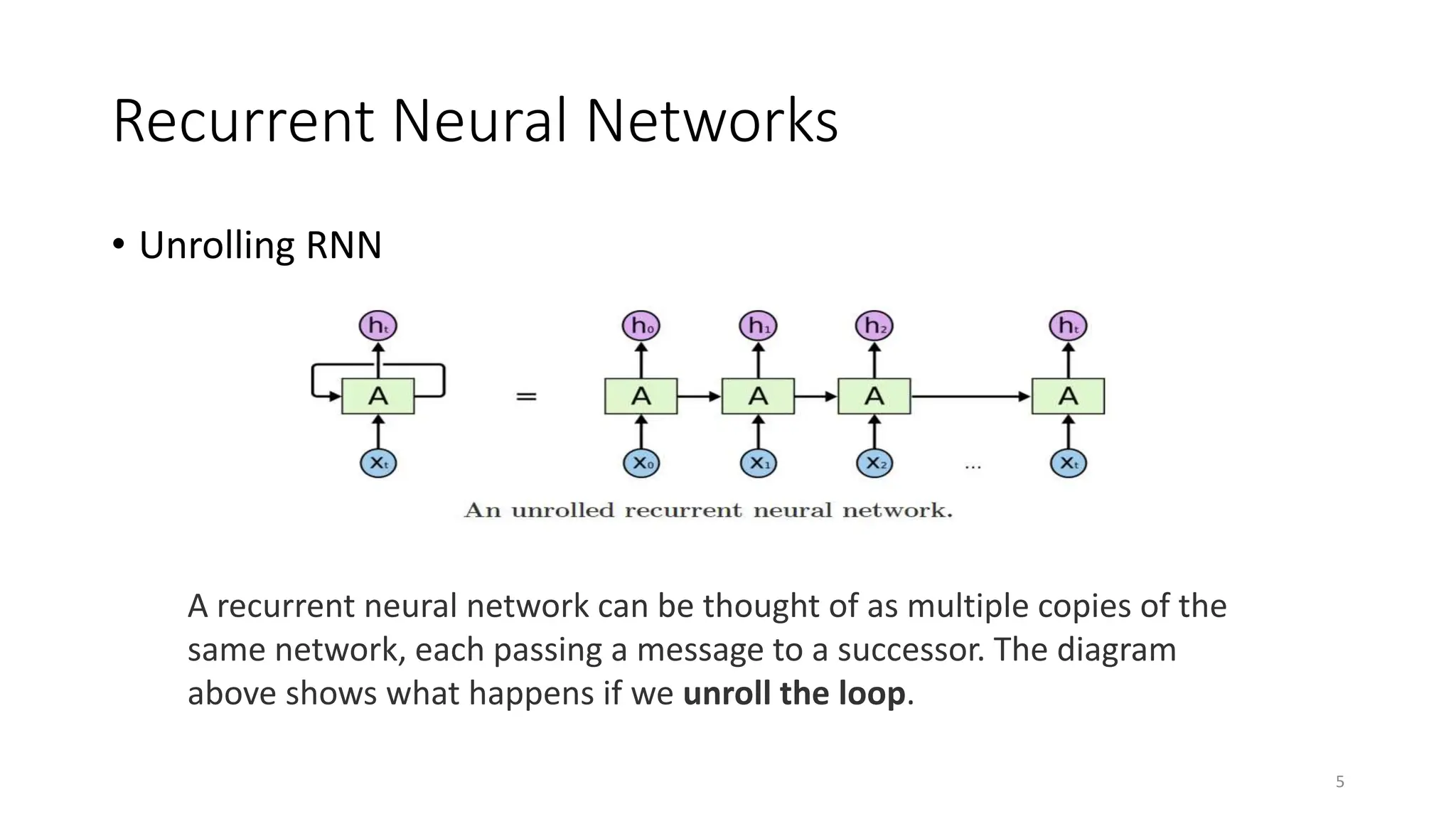
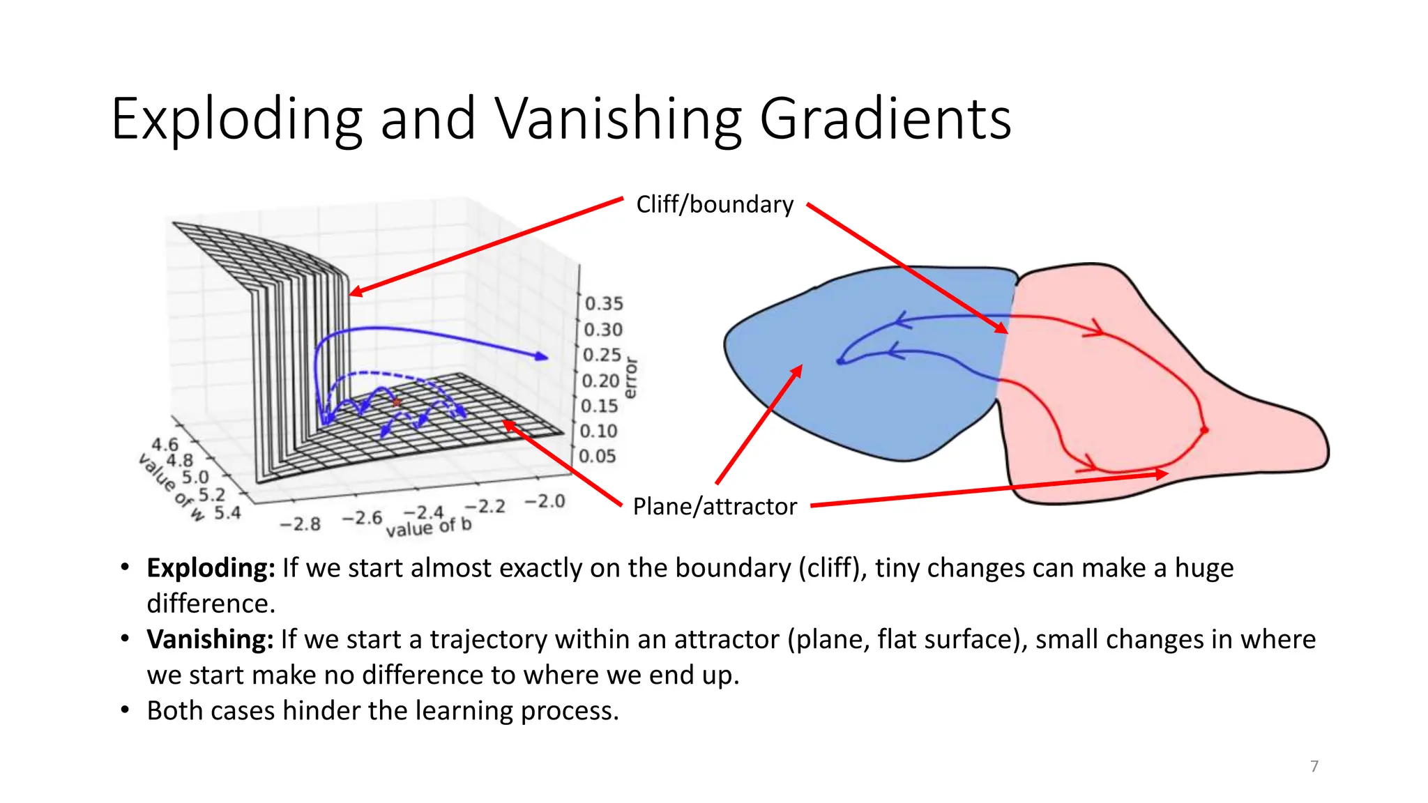
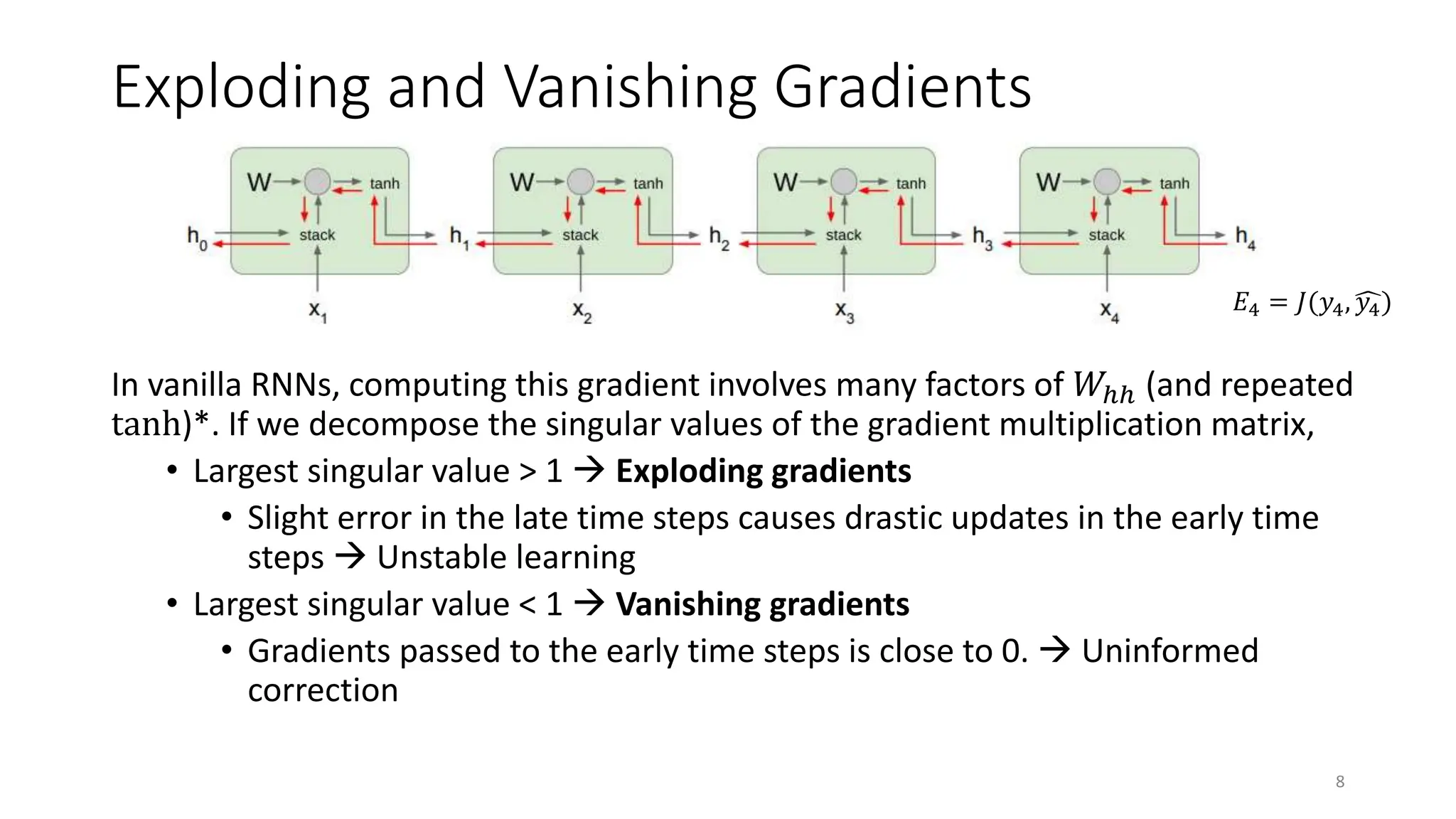
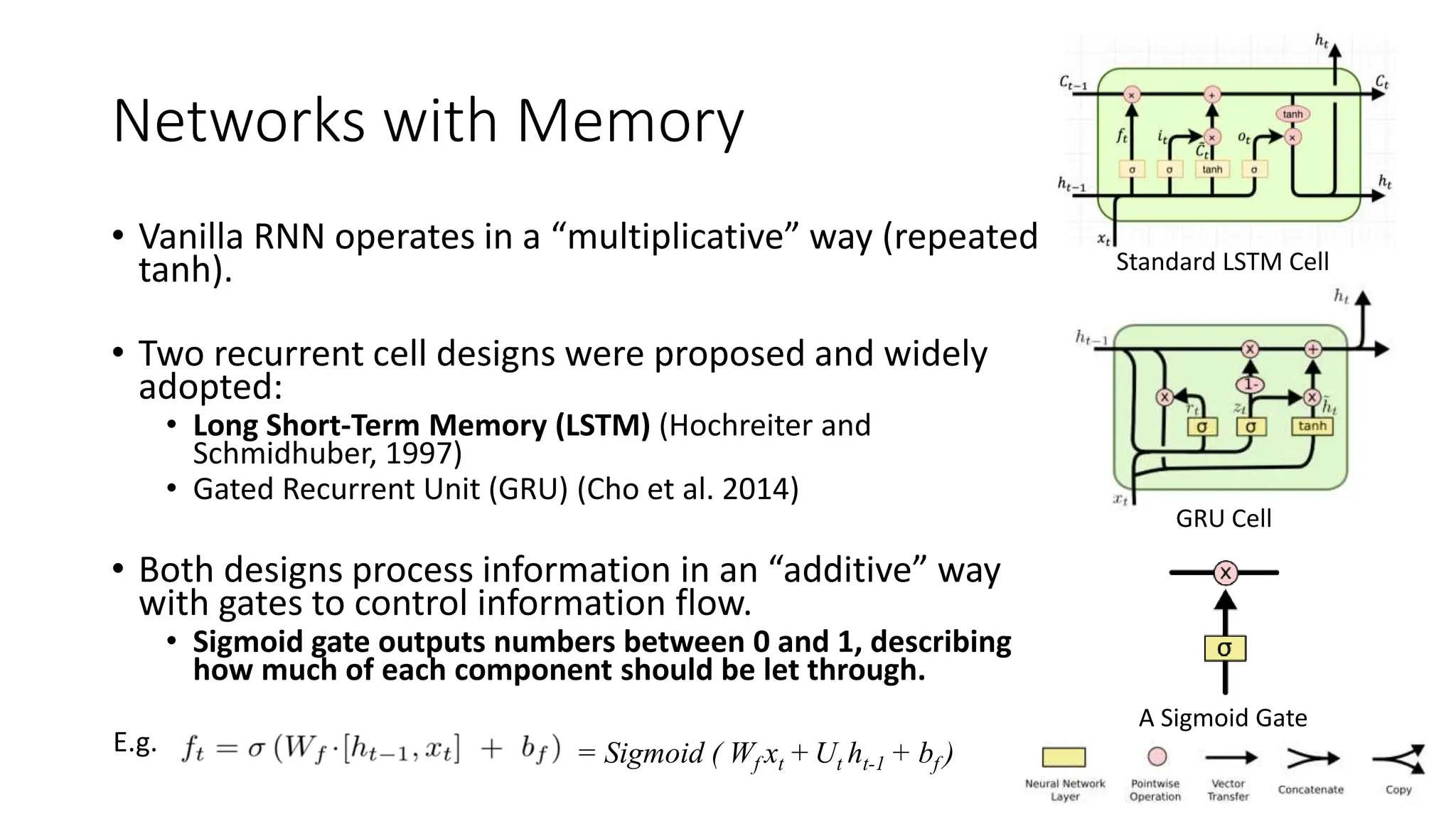
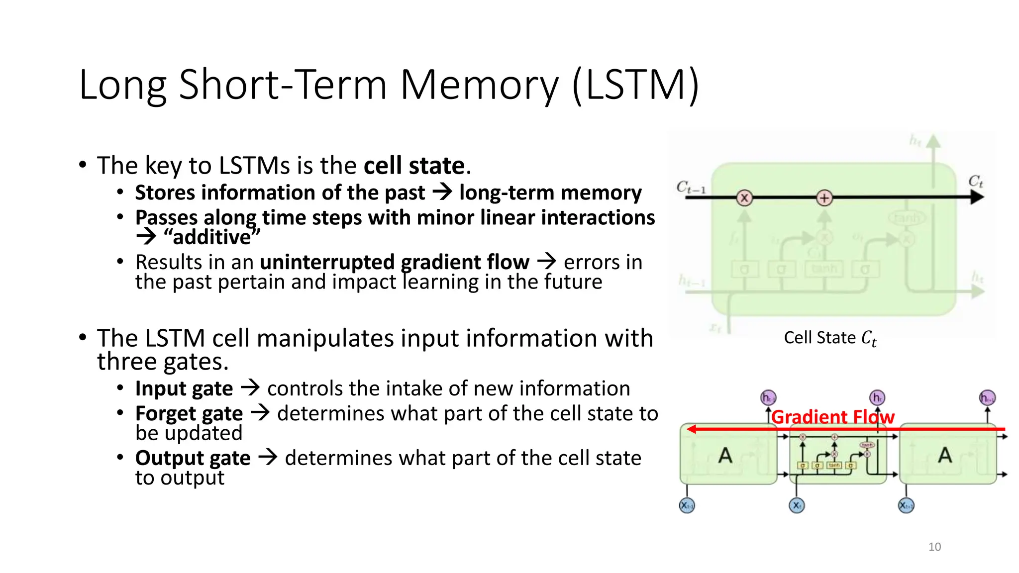
2. Recurrent Neural Networks
• Human brain deals with information streams. Most data is obtained, processed, and
generated sequentially.
• E.g., listening: soundwaves vocabularies/sentences
• E.g., action: brain signals/instructions sequential muscle movements
• Human thoughts have persistence; humans don’t start their thinking from scratch
every second.
• As you read this sentence, you understand each word based on your prior knowledge.
• The applications of standard Artificial Neural Networks (and also Convolutional
Networks) are limited due to:
• They only accepted a fixed-size vector as input (e.g., an image) and produce a fixed-size vector
as output (e.g., probabilities of different classes).
• These models use a fixed amount of computational steps (e.g. the number of layers in the
model).
• Recurrent Neural Networks (RNNs) are a family of neural networks introduced to
learn sequential data.
• Inspired by the temporal-dependent and persistent human thoughts
2
3. Real-life Sequence Learning Applications
• RNNs can be applied to various type of sequential data to learn the
temporal patterns.
• Time-series data (e.g., stock price) Prediction, regression
• Raw sensor data (e.g., signal, voice, handwriting) Labels or text sequences
• Text Label (e.g., sentiment) or text sequence (e.g., translation, summary, answer)
• Image and video Text description (e.g., captions, scene interpretation)
3
Task Input Output
Activity Recognition (Zhu et al. 2018) Sensor Signals Activity Labels
Machine translation (Sutskever et al. 2014) English text French text
Question answering (Bordes et al. 2014) Question Answer
Speech recognition (Graves et al. 2013) Voice Text
Handwriting prediction (Graves 2013) Handwriting Text
Opinion mining (Irsoy et al. 2014) Text Opinion expression
4. Recurrent Neural Networks
• Recurrent Neural Networks are networks with loops,
allowing information to persist.
4
In the above diagram, a chunk of neural
network, A = fW, looks at some
input xt and outputs a value ht. A loop
allows information to be passed from
one step of the network to the next.
Output is to predict a vector ht,
where 𝑜𝑢𝑡𝑝𝑢𝑡 𝑦𝑡 = 𝜑(ℎ𝑡) at some
time steps (t)
5. Recurrent Neural Networks
• Unrolling RNN
5
A recurrent neural network can be thought of as multiple copies of the
same network, each passing a message to a successor. The diagram
above shows what happens if we unroll the loop.
6. Recurrent Neural Networks
• The recurrent structure of RNNs enables the following characteristics:
• Specialized for processing a sequence of values 𝑥 1 , … , 𝑥 𝜏
• Each value 𝑥 𝑖 is processed with the same network A that preserves past information
• Can scale to much longer sequences than would be practical for networks
without a recurrent structure
• Reusing network A reduces the required amount of parameters in the network
• Can process variable-length sequences
• The network complexity does not vary when the input length change
• However, vanilla RNNs suffer from the training difficulty due to exploding and
vanishing gradients.
6
7. Exploding and Vanishing Gradients
• Exploding: If we start almost exactly on the boundary (cliff), tiny changes can make a huge
difference.
• Vanishing: If we start a trajectory within an attractor (plane, flat surface), small changes in where
we start make no difference to where we end up.
• Both cases hinder the learning process.
7
Cliff/boundary
Plane/attractor
8. Exploding and Vanishing Gradients
In vanilla RNNs, computing this gradient involves many factors of 𝑊ℎℎ (and repeated
tanh)*. If we decompose the singular values of the gradient multiplication matrix,
• Largest singular value > 1 Exploding gradients
• Slight error in the late time steps causes drastic updates in the early time
steps Unstable learning
• Largest singular value < 1 Vanishing gradients
• Gradients passed to the early time steps is close to 0. Uninformed
correction
8
𝐸4 = 𝐽(𝑦4, 𝑦4)
9. Networks with Memory
• Vanilla RNN operates in a “multiplicative” way (repeated
tanh).
• Two recurrent cell designs were proposed and widely
adopted:
• Long Short-Term Memory (LSTM) (Hochreiter and
Schmidhuber, 1997)
• Gated Recurrent Unit (GRU) (Cho et al. 2014)
• Both designs process information in an “additive” way
with gates to control information flow.
• Sigmoid gate outputs numbers between 0 and 1, describing
how much of each component should be let through.
9
Standard LSTM Cell
GRU Cell
A Sigmoid Gate
= Sigmoid ( Wf xt + Ut ht-1 + bf )
E.g.
10. Long Short-Term Memory (LSTM)
• The key to LSTMs is the cell state.
• Stores information of the past long-term memory
• Passes along time steps with minor linear interactions
“additive”
• Results in an uninterrupted gradient flow errors in
the past pertain and impact learning in the future
• The LSTM cell manipulates input information with
three gates.
• Input gate controls the intake of new information
• Forget gate determines what part of the cell state to
be updated
• Output gate determines what part of the cell state
to output
10
Gradient Flow
Cell State 𝐶𝑡
11. 11
LSTM: Components & Flow
• LSM unit output
• Output gate units
• Transformed memory cell contents
• Gated update to memory cell units
• Forget gate units
• Input gate units
• Potential input to memory cell
12. Step-by-step LSTM Walk Through
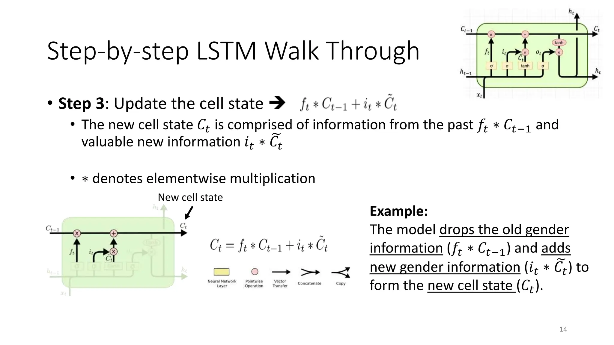
• Step 1: Decide what information to throw away from the cell state
(memory)
• The output of the previous state ℎ𝑡−1 and the new information 𝑥𝑡 jointly
determine what to forget
• ℎ𝑡−1 contains selected features from the memory 𝐶𝑡−1
• Forget gate 𝑓𝑡 ranges between [0, 1]
12
Forget gate
Text processing example:
Cell state may include the gender
of the current subject (ℎ𝑡−1).
When the model observes a new
subject (𝑥𝑡), it may want to forget
(𝑓𝑡 → 0) the old subject in the
memory (𝐶𝑡−1).
13. Step-by-step LSTM Walk Through
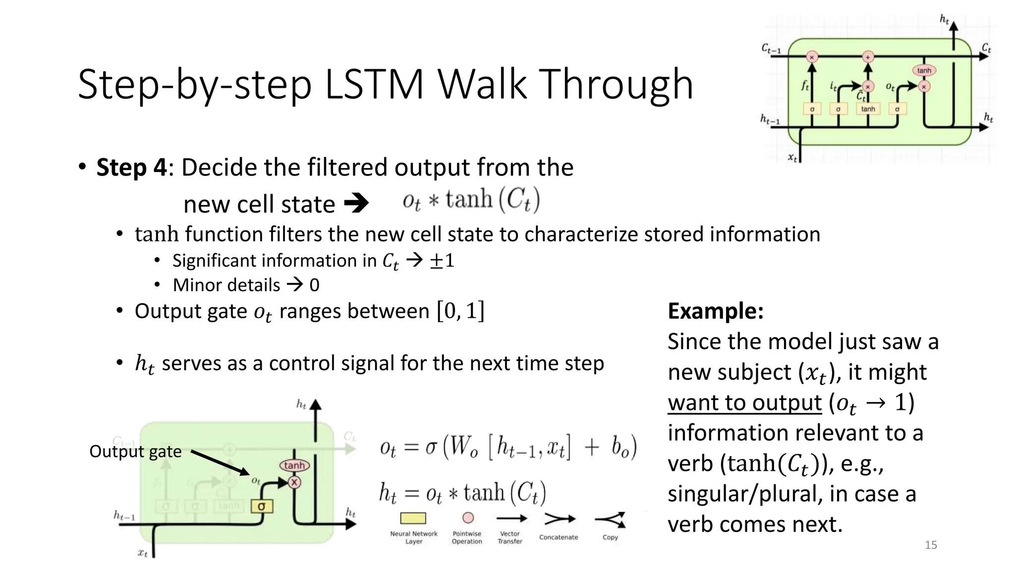
• Step 2: Prepare the updates for the cell state
from input
• An alternative cell state 𝐶𝑡 is created from the new information 𝑥𝑡 with the
guidance of ℎ𝑡−1.
• Input gate 𝑖𝑡 ranges between [0, 1]
13
Input gate Alternative
cell state
Example:
The model may want to add
(𝑖𝑡 → 1) the gender of new
subject (𝐶𝑡) to the cell state to
replace the old one it is
forgetting.
14. Step-by-step LSTM Walk Through
• Step 3: Update the cell state
• The new cell state 𝐶𝑡 is comprised of information from the past 𝑓𝑡 ∗ 𝐶𝑡−1 and
valuable new information 𝑖𝑡 ∗ 𝐶𝑡
• ∗ denotes elementwise multiplication
14
New cell state
Example:
The model drops the old gender
information (𝑓𝑡 ∗ 𝐶𝑡−1) and adds
new gender information (𝑖𝑡 ∗ 𝐶𝑡) to
form the new cell state (𝐶𝑡).
15. Step-by-step LSTM Walk Through
• Step 4: Decide the filtered output from the
new cell state
• tanh function filters the new cell state to characterize stored information
• Significant information in 𝐶𝑡 ±1
• Minor details 0
• Output gate 𝑜𝑡 ranges between 0, 1
• ℎ𝑡 serves as a control signal for the next time step
15
Output gate
Example:
Since the model just saw a
new subject (𝑥𝑡), it might
want to output (𝑜𝑡 → 1)
information relevant to a
verb (tanh(𝐶𝑡)), e.g.,
singular/plural, in case a
verb comes next.
16. Gated Recurrent Unit (GRU)
• GRU is a variation of LSTM that also adopts the gated design.
• Differences:
• GRU uses an update gate 𝒛 to substitute the input and forget gates 𝑖𝑡 and 𝑓𝑡
• Combined the cell state 𝐶𝑡 and hidden state ℎ𝑡 in LSTM as a single cell state ℎ𝑡
• GRU obtains similar performance compared to LSTM with fewer parameters and
faster convergence. (Cho et al. 2014)
16
Update gate: controls the composition of the new state
Reset gate: determines how much old information is needed
in the alternative state ℎ𝑡
Alternative state: contains new information
New state: replace selected old information with
new information in the new state
17. Summary
• LSTM and GRU are RNNs that retain past information and update with
a gated design.
• The “additive” structure avoids vanishing gradient problem.
• RNNs allow flexible architecture designs to adapt to different
sequence learning requirements.
• RNNs have broad real-life applications.
• Text processing, machine translation, signal extraction/recognition, image
captioning
• Mobile health analytics, activity of daily living, senior care
17