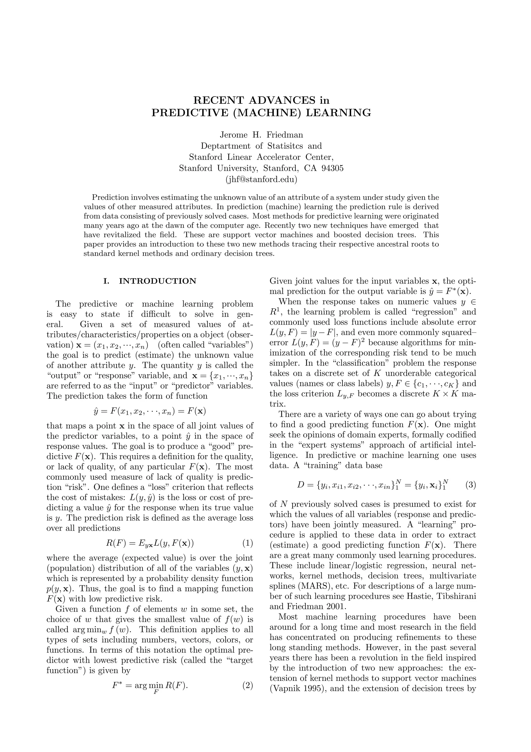
This document provides an introduction to recent advances in predictive machine learning, specifically support vector machines and boosted decision trees. It begins with an overview of predictive learning and common methods. It then describes kernel methods, including how they were extended to support vector machines. Next, it discusses extending decision trees with boosting. The document concludes by comparing support vector machines and boosted decision trees, and noting they are not the only recent advances in machine learning.
Machine learning in science and industry — day 1arogozhnikov
A course of machine learning in science and industry.
- notions and applications
- nearest neighbours: search and machine learning algorithms
- roc curve
- optimal classification and regression
- density estimation
- Gaussian mixtures and EM algorithm
- clustering, an example of clustering in the opera
There are three main types of computer vision models:
1. Discriminative models directly model the posterior Pr(w|x). Inference is straightforward by evaluating this distribution.
2. Generative models model the joint distribution Pr(x,w) or likelihood Pr(x|w). Inference requires more complex calculations using Bayes' rule.
3. For regression problems where the world state w is continuous, discriminative models like linear regression directly model Pr(w|x). For classification where w is discrete, discriminative models like logistic regression model the probability of each class. Generative classification models are difficult to construct.
This document discusses radial basis function networks. It begins by introducing the basic structure of RBF networks, which typically involve an input layer, a hidden layer that applies a nonlinear transformation using radial basis functions, and an output layer with a linear transformation. The document then discusses Cover's theorem, which states that pattern classification problems are more likely to be linearly separable when mapped to a higher-dimensional space through a nonlinear transformation. Several key concepts are introduced, including dichotomies, phi-separable functions, and using hidden functions to map patterns to a hidden feature space.
ANALYTICAL STUDY OF FEATURE EXTRACTION TECHNIQUES IN OPINION MININGcsandit
Although opinion mining is in a nascent stage of development but still the ground is set for dense growth of researches in the field. One of the important activities of opinion mining is to extract opinions of people based on characteristics of the object under study. Feature extraction in opinion mining can be done by various ways like that of clustering, support vector machines
etc. This paper is an attempt to appraise the various techniques of feature extraction. The first part discusses various techniques and second part makes a detailed appraisal of the major techniques used for feature extraction
Analytical study of feature extraction techniques in opinion miningcsandit
Although opinion mining is in a nascent stage of development but still the ground is set for
dense growth of researches in the field. One of the important activities of opinion mining is to
extract opinions of people based on characteristics of the object under study. Feature extraction
in opinion mining can be done by various ways like that of clustering, support vector machines
etc. This paper is an attempt to appraise the various techniques of feature extraction. The first
part discusses various techniques and second part makes a detailed appraisal of the major
techniques used for feature extraction
Machine learning in science and industry — day 2arogozhnikov
- decision trees
- random forest
- Boosting: adaboost
- reweighting with boosting
- gradient boosting
- learning to rank with gradient boosting
- multiclass classification
- trigger in LHCb
- boosting to uniformity and flatness loss
- particle identification
A Maximum Entropy Approach to the Loss Data Aggregation ProblemErika G. G.
This document discusses using a maximum entropy approach to model loss distributions for operational risk modeling. It begins by motivating the need to accurately model loss distributions given challenges with limited datasets, including heavy tails and dependence between risks. It then provides an overview of the loss distribution approach commonly used in operational risk modeling and its limitations. The document introduces the maximum entropy approach, which frames the problem as maximizing entropy subject to moment constraints. It discusses using the Laplace transform of loss distributions to compress information into moments and how these can be estimated from sample data or fitted distributions to serve as constraints for the maximum entropy approach.
This document provides an introduction to neural networks. It begins with an outline covering statistical machine learning concepts like underfitting, overfitting and consistency. It then discusses multi-layer perceptrons, the basic building blocks of neural networks. It covers how perceptrons are presented, their theoretical properties, and how learning occurs. Finally, it provides an overview of deep neural networks and convolutional neural networks. The goal is to introduce fundamental concepts in neural networks from statistical learning to modern deep learning architectures.
Conventional tools in array signal processing have traditionally relied on the availability of a large number of samples acquired at each sensor or array element (antenna, hydrophone, microphone, etc.). Large sample size assumptions typically guarantee the consistency of estimators, detectors, classifiers and multiple other widely used signal processing procedures. However, practical scenario and array mobility conditions, together with the need for low latency and reduced scanning times, impose strong limits on the total number of observations that can be effectively processed. When the number of collected samples per sensor is small, conventional large sample asymptotic approaches are not relevant anymore. Recently, large random matrix theory tools have been proposed in order to address the small sample support problem in array signal processing. In fact, it has been shown that the most important and longstanding problems in this field can be reformulated and studied according to this asymptotic paradigm. By exploiting the latest advances in large random matrix theory and high dimensional statistics, a novel and unconventional methodology can be established, which provides an unprecedented treatment of the finite sample-per-sensor regime. In this talk, we will see that random matrix theory establishes a unifying framework for the study of array signal processing techniques under the constraint of a small number of observations per sensor, which has radically changed the way in which array processing methodologies have been traditionally established. We will show how this unconventional way of revisiting classical array processing has lead to major advances in the design and analysis of signal processing techniques for multidimensional observations.
This document provides an overview of classification in machine learning. It discusses supervised learning and the classification process. It describes several common classification algorithms including k-nearest neighbors, Naive Bayes, decision trees, and support vector machines. It also covers performance evaluation metrics like accuracy, precision and recall. The document uses examples to illustrate classification tasks and the training and testing process in supervised learning.
(研究会輪読) Facial Landmark Detection by Deep Multi-task LearningMasahiro Suzuki
The document summarizes a research paper on facial landmark detection using deep multi-task learning. It proposes a Tasks-Constrained Deep Convolutional Network (TCDCN) that uses facial landmark detection as the main task and related auxiliary tasks like pose estimation and attribute inference to improve performance. The TCDCN learns shared representations across tasks using a deep convolutional network. It introduces task-wise early stopping to halt learning on auxiliary tasks that reach optimal performance early to avoid overfitting and improve convergence on the main task of landmark detection. Experimental results showed the proposed approach outperformed existing methods.
Combining Models - In this slides, we look at a way to combine the answers form various weak classifiers to build a robust classifier. At the slides we look at the following subjects:
1.- Model Combination Vs Bayesian Model
2.- Bootstrap Data Sets
And the cherry on the top the AdaBoost
The document summarizes statistical pattern recognition techniques. It is divided into 9 sections that cover topics like dimensionality reduction, classifiers, classifier combination, and unsupervised classification. The goal of pattern recognition is supervised or unsupervised classification of patterns based on features. Dimensionality reduction aims to reduce the number of features to address the curse of dimensionality when samples are limited. Multiple classifiers can be combined through techniques like stacking, bagging, and boosting. Unsupervised classification uses clustering algorithms to construct decision boundaries without labeled training data.
This document discusses cluster validity, which is a method for quantitatively evaluating the results of a clustering algorithm. Cluster validity is important because clustering algorithms sometimes impose structure on data even when no natural clusters exist. The document outlines different techniques for cluster validity testing, including hypothesis testing, Monte Carlo techniques, and bootstrapping. It also discusses the concept of a power function, which compares the effectiveness of different statistical tests for validating clustering results. The overall goal of cluster validity is to determine the appropriate number of clusters and whether the data exhibits a genuine clustering structure.
This document discusses challenges in comparing structured models using cross-validation. It presents a decision-theoretic framework for model assessment and selection based on expected predictive loss. Different methods for estimating predictive loss are discussed, including k-fold cross-validation which is used to estimate the predictive loss of various multilevel models for a dataset from the Cooperative Congressional Election Survey with deeply nested demographic variables.
The Sample Average Approximation Method for Stochastic Programs with Integer ...SSA KPI
The document describes a sample average approximation method for solving stochastic programs with integer recourse. It approximates the expected recourse cost function using a sample average based on a sample of scenarios. It shows that as the sample size increases, the solution to the sample average approximation problem converges exponentially fast to the optimal solution of the true stochastic program. It also describes statistical and deterministic techniques for validating candidate solutions. Preliminary computational results applying this method are also mentioned.
Uncertainty Awareness in Integrating Machine Learning and Game TheoryRikiya Takahashi
This document discusses integrating machine learning and game theory while accounting for uncertainty. It provides an example of previous work predicting travel time distribution on a road network using taxi data. It also discusses functional approximation in reinforcement learning, noting that techniques like deep learning can better represent functions with fewer parameters compared to nonparametric models like random forests. The document emphasizes avoiding unnecessary intermediate estimation steps and using approaches like fitted Q-iteration that are robust to estimation errors from small datasets.
The document discusses the principle of maximum entropy. It explains that maximum entropy is an approach for making probability assignments where the assigned probability distribution should have the largest entropy or uncertainty possible, subject to whatever information is known. It describes applications of maximum entropy modeling such as part-of-speech tagging and logistic regression. Maximum entropy and maximum likelihood methods are related as they both aim to make distributions as uniform as possible based on available information.
This document describes a statistical framework for interactive image category search based on mental matching. The framework allows a user to search an unstructured image database for a target category that exists only as a "mental picture" by providing feedback on displayed image sets. At each iteration, the system selects images to maximize the information gained from the user's response. The goal is to minimize the number of iterations needed to display an image from the target category. Experiments showed the approach was effective on databases containing tens of thousands of images across several semantic categories.
Here a Review of the Combination of Machine Learning models from Bayesian Averaging, Committees to Boosting... Specifically An statistical analysis of Boosting is done
1. The document discusses the author's research in three areas: graph-based clustering methods, approximate Bayesian computation (ABC), and Bayesian computation using empirical likelihood.
2. For graph-based clustering, the author presents asymptotic results for spectral clustering as the number of data points and bandwidth approach infinity.
3. For ABC, the author discusses sequential ABC algorithms and challenges of model choice and high-dimensional summary statistics. Machine learning methods are proposed to analyze simulated ABC data.
4. For empirical likelihood, the author proposes using it for Bayesian computation when the likelihood is intractable and simulation is infeasible, as it provides correct confidence intervals unlike composite likelihoods.
The document introduces Bayesian classifiers and the naive Bayes model. It discusses key concepts like likelihood, prior probability, and evidence. The naive Bayes model uses Bayes' theorem to calculate the posterior probability of class membership given observed data. The optimal Bayesian classification rule is to assign the data point to the class with the highest posterior probability. Minimizing classification error is achieved by selecting the decision boundary that minimizes the sum of the error probabilities for each class.
An Importance Sampling Approach to Integrate Expert Knowledge When Learning B...NTNU
The introduction of expert knowledge when learning Bayesian Networks from data is known to be an excellent approach to boost the performance of automatic learning methods, specially when the data is scarce. Previous approaches for this problem based on Bayesian statistics introduce the expert knowledge modifying the prior probability distributions. In this study, we propose a new methodology based on Monte Carlo simulation which starts with non-informative priors and requires knowledge from the expert a posteriori, when the simulation ends. We also explore a new Importance Sampling method for Monte Carlo simulation and the definition of new non-informative priors for the structure of the network. All these approaches are experimentally validated with five standard Bayesian networks.
Read more:
http://link.springer.com/chapter/10.1007%2F978-3-642-14049-5_70
Composing graphical models with neural networks for structured representatio...Jeongmin Cha
This presentation discusses the Structural Variational Autoencoder (SVAE) model, which combines graphical models and neural networks. SVAE uses neural networks to model observations and produce dense low-dimensional representations, while also explicitly representing discrete mixture components through a graphical model. This allows for structured probabilistic representations and fast exact inference. SVAE leverages the conjugacy property between the prior and posterior distributions, which aids Bayesian inference and makes the marginal likelihood tractable. The model is demonstrated on a mouse behavior video segmentation task.
Reinforcement learning (RL) involves learning goal-directed behavior from rewards and punishments. RL algorithms allow agents to learn by experiencing interactions with an environment to maximize rewards. Key concepts in RL include states, actions, rewards, value functions, and policies. Temporal difference (TD) learning methods like TD(0) provide incremental updates to value functions by bootstrapping from the value of future states, allowing agents to learn online without waiting for episodes to finish.
This document is a resume for Amit Sethi summarizing his professional experience and qualifications. It outlines his objective to obtain a research and development position in industry. It then details his education at the University of Illinois at Urbana-Champaign where he is pursuing a PhD in Electrical and Computer Engineering, as well as a previous degree from Indian Institute of Technology. His experience includes research in machine learning, computer vision, and video processing. He has several publications and awards and is skilled in programming languages such as C++.
This document provides a listing and brief descriptions of working papers from 2000. It includes 12 papers with titles and short 1-2 paragraph summaries of each paper's topic or focus. The papers cover a range of topics related to text mining, machine learning, data compression, knowledge discovery, and user interfaces for developing classifiers.
The document discusses two NSF-funded research projects on intelligence and security informatics:
1. A project to filter and monitor message streams to detect "new events" and changes in topics or activity levels. It describes the technical challenges and components of automatic message processing.
2. A project called HITIQA to develop high-quality interactive question answering. It describes the team members and key research issues like question semantics, human-computer dialogue, and information quality metrics.
SVMlight is an implementation of Support Vector Machines (SVMs) that can be used for classification, regression, and preference ranking problems. It has efficient memory usage and can handle large datasets. The source code and binaries can be downloaded for various operating systems. SVMlight consists of a learning module (svm_learn) that trains models from input data, and a classification module (svm_classify) that applies trained models to make predictions on new data. The svm_learn module is called with options to specify the problem type, tradeoff parameter, and other settings. Models are saved for use by svm_classify.
The document discusses machine learning techniques for multivariate data analysis using the TMVA toolkit. It describes several common classification problems in high energy physics (HEP) and summarizes several machine learning algorithms implemented in TMVA for supervised learning, including rectangular cut optimization, likelihood methods, neural networks, boosted decision trees, support vector machines and rule ensembles. It also discusses challenges like nonlinear correlations between input variables and techniques for data preprocessing and decorrelation.
This document provides an introduction to machine learning, covering key topics such as what machine learning is, common learning algorithms and applications. It discusses linear models, kernel methods, neural networks, decision trees and more. It also addresses challenges in machine learning like balancing fit and robustness, and evaluating model performance using techniques like ROC curves. The goal of machine learning is to build models that can learn from data to make predictions or decisions.
This document summarizes support vector machines (SVMs), a machine learning technique for classification and regression. SVMs find the optimal separating hyperplane that maximizes the margin between positive and negative examples in the training data. This is achieved by solving a convex optimization problem that minimizes a quadratic function under linear constraints. SVMs can perform non-linear classification by implicitly mapping inputs into a higher-dimensional feature space using kernel functions. They have applications in areas like text categorization due to their ability to handle high-dimensional sparse data.
This document provides an overview of machine learning techniques for classification and anomaly detection. It begins with an introduction to machine learning and common tasks like classification, clustering, and anomaly detection. Basic classification techniques are then discussed, including probabilistic classifiers like Naive Bayes, decision trees, instance-based learning like k-nearest neighbors, and linear classifiers like logistic regression. The document provides examples and comparisons of these different methods. It concludes by discussing anomaly detection and how it differs from classification problems, noting challenges like having few positive examples of anomalies.
Artificial intelligence is the simulation of human intelligence processes by machines, especially computer systems. Specific applications of AI include expert systems, natural language processing, speech recognition and machine vision.
Classifiers are algorithms that map input data to categories in order to build models for predicting unknown data. There are several types of classifiers that can be used including logistic regression, decision trees, random forests, support vector machines, Naive Bayes, and neural networks. Each uses different techniques such as splitting data, averaging predictions, or maximizing margins to classify data. The best classifier depends on the problem and achieving high accuracy, sensitivity, and specificity.
Improving Performance of Back propagation Learning Algorithmijsrd.com
The standard back-propagation algorithm is one of the most widely used algorithm for training feed-forward neural networks. One major drawback of this algorithm is it might fall into local minima and slow convergence rate. Natural gradient descent is principal method for solving nonlinear function is presented and is combined with the modified back-propagation algorithm yielding a new fast training multilayer algorithm. This paper describes new approach to natural gradient learning in which the number of parameters necessary is much smaller than the natural gradient algorithm. This new method exploits the algebraic structure of the parameter space to reduce the space and time complexity of algorithm and improve its performance.
Surrogate models emulate expensive computer simulations. The objective is to approximate a function, $f$, of $d$ variables to a given tolerance, $\varepsilon$, using as few function values as possible, preferably $O(d)$. We explain how tractability theory provides lower bounds on the number of function values required for any possible method. We also propose method for sampling $f$ and approximating $f$ that achieves this objective and the kind of underlying structure that $f$ must have for success.
This document proposes a new gene selection algorithm using Bayesian classification. The algorithm begins with an empty gene subset and iteratively adds genes that provide the maximum information to the subset. Genes are selected until no additional genes improve the classification accuracy. A Bayesian classifier is used to evaluate the contribution of each gene. The proposed algorithm is tested on several publicly available gene expression datasets and shown to provide promising results compared to other gene selection methods.
Radial Basis Function Neural Network (RBFNN), Induction Motor, Vector control...cscpconf
Although opinion mining is in a nascent stage of development but still the ground is set for dense growth of researches in the field. One of the important activities of opinion mining is to
extract opinions of people based on characteristics of the object under study. Feature extraction in opinion mining can be done by various ways like that of clustering, support vector machines
etc. This paper is an attempt to appraise the various techniques of feature extraction. The first part discusses various techniques and second part makes a detailed appraisal of the major techniques used for feature extraction.
The document discusses various machine learning techniques including k-nearest neighbors, which classifies new data based on its similarity to existing examples; Naive Bayes classifiers, which use Bayes' theorem to classify items based on the presence or absence of features; and decision trees, which classify items by sorting them based on the results of tests on their features and dividing them into branches. Reinforcement learning is also covered, where an agent learns through trial-and-error interactions with an environment by receiving rewards or penalties for actions.
This document discusses using Lagrange interpolation to estimate missing values in datasets. It begins with an introduction to missing data problems and common techniques for handling missing values like deletion, mean substitution, and more. It then explains Lagrange interpolation, which uses known data points to estimate values at unknown points. The algorithm for Lagrange interpolation is presented. An example using years of experience and salary data to estimate salary for 10 years of experience is shown. The document concludes that Lagrange interpolation can be used to estimate missing values in preprocessing if the relationship between attributes is uniform. Limitations are noted if the relationship is not uniform.
2.6 support vector machines and associative classifiers revisedKrish_ver2
Support vector machines (SVMs) are a type of supervised machine learning model that can be used for both classification and regression analysis. SVMs work by finding a hyperplane in a multidimensional space that best separates clusters of data points. Nonlinear kernels can be used to transform input data into a higher dimensional space to allow for the detection of complex patterns. Associative classification is an alternative approach that uses association rule mining to generate rules describing attribute relationships that can then be used for classification.
This document presents a method for applying random matrix theory to analyze deep neural networks using nonlinear activations. The key results are:
1) The moments method is used to derive a quartic equation that the Stieltjes transform of the Gram matrix YTY satisfies, where Y=f(WX) and W,X are random matrices and f is a nonlinear activation.
2) This allows computing properties of the Gram matrix like its limiting spectral distribution and the training loss of a random feature network.
3) Certain activations preserve the eigenvalue distribution of the data covariance matrix XTX, analogous to batch normalization. These activations may improve training and are a new class worthy of further study.
The document discusses machine learning concepts including supervised and unsupervised learning algorithms like clustering, dimensionality reduction, and classification. It also covers parallel computing strategies for machine learning like partitioning problems across distributed memory systems.
The document discusses machine learning concepts including supervised and unsupervised learning algorithms like clustering, dimensionality reduction, and classification. It also covers parallel computing strategies for machine learning like partitioning problems across distributed memory architectures.
The document discusses machine learning concepts including supervised and unsupervised learning algorithms like clustering, dimensionality reduction, and classification. It also covers parallel computing strategies for machine learning like partitioning problems across systems.
The document discusses machine learning concepts including supervised and unsupervised learning algorithms like clustering, dimensionality reduction, and classification. It also covers parallel computing strategies for machine learning like partitioning problems across distributed memory systems.
Similar to RECENT ADVANCES in PREDICTIVE (MACHINE) LEARNING (20)
Este documento analiza el modelo de negocio de YouTube. Explica que YouTube y otros sitios de video online representan un nuevo modelo de negocio para contenidos audiovisuales debido al cambio en los hábitos de consumo causado por las nuevas tecnologías. Describe cómo YouTube aprovecha la participación de los usuarios para mejorar continuamente y atraer una audiencia diferente a la de los medios tradicionales.
The defense was successful in portraying Michael Jackson favorably to the jury in several ways:
1) They dressed Jackson in ornate costumes that conveyed images of purity, innocence, and humility.
2) Jackson was shown entering the courtroom as if on a red carpet, emphasizing his celebrity status.
3) Jackson appeared vulnerable, childlike, and in declining health during the trial, eliciting sympathy from jurors.
4) Defense attorney Tom Mesereau effectively presented a coherent narrative of Jackson as a victim and portrayed Neverland as a place of refuge, undermining the prosecution's arguments.
Michael Jackson was born in 1958 in Gary, Indiana and rose to fame in the 1960s as the lead singer of The Jackson 5, topping music charts in the 1970s. As a solo artist in the 1980s, his album Thriller broke music records. In the 1990s and 2000s, Jackson faced several legal issues related to child abuse allegations while continuing to release music. He married Lisa Marie Presley and Debbie Rowe and had two children before his death in 2009.
Popular Reading Last Updated April 1, 2010 Adams, Lorraine The ...butest
This document appears to be a list of popular books from various authors. It includes over 150 book titles across many genres such as fiction, non-fiction, memoirs, and novels. The books cover a wide range of topics from politics to cooking to autobiographies.
The prosecution lost the Michael Jackson trial due to several key mistakes and weaknesses in their case:
1) The lead prosecutor, Thomas Sneddon, was too personally invested in the case against Jackson, having pursued him for over a decade without success.
2) Sneddon's opening statement was disorganized and weak, failing to effectively outline the prosecution's case.
3) The accuser's mother was not credible and damaged the prosecution's case through her erratic testimony, history of lies and con artist behavior.
4) Many prosecution witnesses were not credible due to prior lawsuits against Jackson, debts owed to him, or having been fired by him. Several witnesses even took the Fifth Amendment.
Here are three examples of public relations from around the world:
1. The UK government's "Be Clear on Cancer" campaign which aims to raise awareness of cancer symptoms and encourage early diagnosis.
2. Samsung's global brand marketing and sponsorship activities which aim to increase brand awareness and favorability of Samsung products worldwide.
3. The Brazilian government's efforts to improve its international image and relations with other countries through strategic communication and diplomacy.
The three most important functions of public relations are:
1. Media relations because the media is how most organizations reach their key audiences. Strong media relationships are crucial.
2. Writing, because written communication is at the core of public relations and how most information is
Michael Jackson Please Wait... provides biographical information about Michael Jackson including his birthdate, birthplace, parents, height, interests, idols, favorite foods, films, and more. It discusses his background, career highlights including influential albums like Thriller, and films he appeared in such as The Wiz and Moonwalker. The document contains photos and details about Jackson's life and illustrious music career.
The MYnstrel Free Press Volume 2: Economic Struggles, Meet Jazzbutest
The document discusses the process of manufacturing celebrity and its negative byproducts. It argues that celebrities are rarely the best in their individual pursuits like singing, dancing, etc. but become famous due to being products of a system controlled by wealthy elites. This system stifles opportunities for worthy artists and creates feudalism. The document also asserts that manufactured celebrities should not be viewed as role models due to behaviors like drug abuse and narcissism that result from the celebrity-making process.
Michael Jackson was a child star who rose to fame with the Jackson 5 in the late 1960s and early 1970s. As a solo artist in the 1970s and 1980s, he had immense commercial success with albums like Off the Wall, Thriller, and Bad, which featured hit singles and groundbreaking music videos. However, his career and public image were plagued by controversies related to allegations of child sexual abuse in the 1990s and 2000s. He continued recording and performing but faced ongoing media scrutiny into his private life until his death in 2009.
Social Networks: Twitter Facebook SL - Slide 1butest
The document discusses using social networking tools like Twitter and Facebook in K-12 education. Twitter allows students and teachers to share short updates and can be used to give parents a window into classroom activities. Facebook allows targeted advertising that could be used to promote educational activities. Both tools could help facilitate communication between schools and communities if used properly while managing privacy and security concerns.
Facebook has over 300 million active users who log on daily, and allows brands to create public profile pages to interact with users. Pages are for brands and organizations only, while groups can be made by any user about any topic. Pages do not show admin names and have no limits on fans, while groups display admin names and are limited to 5,000 members. Content on pages should aim to provoke action from subscribers and establish a regular posting schedule using a conversational tone.
Executive Summary Hare Chevrolet is a General Motors dealership ...butest
Hare Chevrolet is a car dealership located in Noblesville, Indiana that has successfully used social media platforms like Twitter, Facebook, and YouTube to create a positive brand image. They invest significant time interacting directly with customers online to foster a sense of community rather than overtly advertising. As a result, Hare Chevrolet has built a large, engaged audience on social media and serves as a model for how brands can use online presences strategically.
Welcome to the Dougherty County Public Library's Facebook and ...butest
This document provides instructions for signing up for Facebook and Twitter accounts. It outlines the sign up process for both platforms, including filling out forms with name, email, password and other details. It describes how the platforms will then search for friends and suggest people to connect with. It also explains how to search for and follow the Dougherty County Public Library page on both Facebook and Twitter once signed up. The document concludes by thanking participants and providing a contact for any additional questions.
Paragon Software announces the release of Paragon NTFS for Mac OS X 8.0, which provides full read and write access to NTFS partitions on Macs. It is the fastest NTFS driver on the market, achieving speeds comparable to native Mac file systems. Paragon NTFS for Mac 8.0 fully supports the latest Mac OS X Snow Leopard operating system in 64-bit mode and allows easy transfer of files between Windows and Mac partitions without additional hardware or software.
This document provides compatibility information for Olympus digital products used with Macintosh OS X. It lists various digital cameras, photo printers, voice recorders, and accessories along with their connection type and any notes on compatibility. Some products require booting into OS 9.1 for software compatibility or do not support devices that need a serial port. Drivers and software are available for download from Olympus and other websites for many products to enable use with OS X.
To use printers managed by the university's Information Technology Services (ITS), students and faculty must install the ITS Remote Printing software on their Mac OS X computer. This allows them to add network printers, log in with their ITS account credentials, and print documents while being charged per page to funds in their pre-paid ITS account. The document provides step-by-step instructions for installing the software, adding a network printer, and printing to that printer from any internet connection on or off campus. It also explains the pay-in-advance printing payment system and how to check printing charges.
The document provides an overview of the Mac OS X user interface for beginners, including descriptions of the desktop, login screen, desktop elements like the dock and hard disk, and how to perform common tasks like opening files and folders. It also addresses frequently asked questions for Windows users switching to Mac OS X, such as where documents are stored, how to save or find documents, and what the equivalent of the C: drive is in Mac OS X. The document concludes with sections on file management tasks like creating and deleting folders, organizing files within applications, using Spotlight search, and an overview of the Dashboard feature.
This document provides a checklist for securing Mac OS X version 10.5, focusing on hardening the operating system, securing user accounts and administrator accounts, enabling file encryption and permissions, implementing intrusion detection, and maintaining password security. It describes the Unix infrastructure and security framework that Mac OS X is built on, leveraging open source software and following the Common Data Security Architecture model. The checklist can be used to audit a system or harden it against security threats.
This document summarizes a course on web design that was piloted in the summer of 2003. The course was a 3 credit course that met 4 times a week for lectures and labs. It covered topics such as XHTML, CSS, JavaScript, Photoshop, and building a basic website. 18 students from various majors enrolled. Student and instructor evaluations found the course to be very successful overall, though some improvements were suggested like ensuring proper software and pairing programming/non-programming students. The document also discusses implications of incorporating web design material into existing computer science curriculums.
1. RECENT ADVANCES in
PREDICTIVE (MACHINE) LEARNING
Jerome H. Friedman
Deptartment of Statisitcs and
Stanford Linear Accelerator Center,
Stanford University, Stanford, CA 94305
(jhf@stanford.edu)
Prediction involves estimating the unknown value of an attribute of a system under study given the
values of other measured attributes. In prediction (machine) learning the prediction rule is derived
from data consisting of previously solved cases. Most methods for predictive learning were originated
many years ago at the dawn of the computer age. Recently two new techniques have emerged that
have revitalized the field. These are support vector machines and boosted decision trees. This
paper provides an introduction to these two new methods tracing their respective ancestral roots to
standard kernel methods and ordinary decision trees.
I. INTRODUCTION Given joint values for the input variables x, the opti-
mal prediction for the output variable is y = F ∗ (x).
ˆ
The predictive or machine learning problem When the response takes on numeric values y ∈
is easy to state if difficult to solve in gen- R1 , the learning problem is called “regression” and
eral. Given a set of measured values of at- commonly used loss functions include absolute error
tributes/characteristics/properties on a object (obser- L(y, F ) = |y − F |, and even more commonly squared–
vation) x = (x1 , x2 , ···, xn ) (often called “variables”) error L(y, F ) = (y − F )2 because algorithms for min-
the goal is to predict (estimate) the unknown value imization of the corresponding risk tend to be much
of another attribute y. The quantity y is called the simpler. In the “classification” problem the response
“output” or “response” variable, and x = {x1 , ···, xn } takes on a discrete set of K unorderable categorical
are referred to as the “input” or “predictor” variables. values (names or class labels) y, F ∈ {c1 , · · ·, cK } and
The prediction takes the form of function the loss criterion Ly,F becomes a discrete K × K ma-
trix.
y = F (x1 , x2 , · · ·, xn ) = F (x)
ˆ There are a variety of ways one can go about trying
that maps a point x in the space of all joint values of to find a good predicting function F (x). One might
the predictor variables, to a point y in the space of
ˆ seek the opinions of domain experts, formally codified
response values. The goal is to produce a “good” pre- in the “expert systems” approach of artificial intel-
dictive F (x). This requires a definition for the quality, ligence. In predictive or machine learning one uses
or lack of quality, of any particular F (x). The most data. A “training” data base
commonly used measure of lack of quality is predic-
tion “risk”. One defines a “loss” criterion that reflects D = {yi , xi1 , xi2 , · · ·, xin }1 = {yi , xi }N
N
1 (3)
the cost of mistakes: L(y, y ) is the loss or cost of pre-
ˆ
dicting a value y for the response when its true value
ˆ of N previously solved cases is presumed to exist for
is y. The prediction risk is defined as the average loss which the values of all variables (response and predic-
over all predictions tors) have been jointly measured. A “learning” pro-
cedure is applied to these data in order to extract
R(F ) = Eyx L(y, F (x)) (1) (estimate) a good predicting function F (x). There
where the average (expected value) is over the joint are a great many commonly used learning procedures.
(population) distribution of all of the variables (y, x) These include linear/logistic regression, neural net-
which is represented by a probability density function works, kernel methods, decision trees, multivariate
p(y, x). Thus, the goal is to find a mapping function splines (MARS), etc. For descriptions of a large num-
F (x) with low predictive risk. ber of such learning procedures see Hastie, Tibshirani
Given a function f of elements w in some set, the and Friedman 2001.
choice of w that gives the smallest value of f (w) is Most machine learning procedures have been
called arg minw f (w). This definition applies to all around for a long time and most research in the field
types of sets including numbers, vectors, colors, or has concentrated on producing refinements to these
functions. In terms of this notation the optimal pre- long standing methods. However, in the past several
dictor with lowest predictive risk (called the “target years there has been a revolution in the field inspired
function”) is given by by the introduction of two new approaches: the ex-
tension of kernel methods to support vector machines
F ∗ = arg min R(F ). (2) (Vapnik 1995), and the extension of decision trees by
F
2. 2 PHYSTAT2003, SLAC, Stanford, Calfornia, September 8-11, 2003
boosting (Freund and Schapire 1996, Friedman 2001). (4) (5) approaches the optimal predicting target func-
It is the purpose of this paper to provide an introduc- tion (2), FN (x) → F ∗ (x), provided the value chosen
tion to these new developments. First the classic ker- for the scale parameter σ as a function of N ap-
nel and decision tree methods are introduced. Then proaches zero, σ(N ) → 0, at a slower rate than 1/N .
the extension of kernels to support vector machines is This result holds for almost any distance function
described, followed by a description of applying boost- d(x, x ); only very mild restrictions (such as convex-
ing to extend decision tree methods. Finally, similari- ity) are required. Another advantage of kernel meth-
ties and differences between these two approaches will ods is that no training is required to build a model; the
be discussed. training data set is the model. Also, the procedure is
Although arguably the most influential recent de- conceptually quite simple and easily explained.
velopments, support vector machines and boosting are Kernel methods suffer from some disadvantages
not the only important advances in machine learning that have kept them from becoming highly used in
in the past several years. Owing to space limitations practice, especially in data mining applications. Since
these are the ones discussed here. There have been there is no model, they provide no easily understood
other important developments that have considerably model summary. Thus, they cannot be easily inter-
advanced the field as well. These include (but are not preted. There is no way to discern how the function
limited to) the bagging and random forest techniques FN (x) (4) depends on the respective predictor vari-
of Breiman 1996 and 2001 that are somewhat related ables x. Kernel methods produce a “black–box” pre-
to boosting, and the reproducing kernel Hilbert space diction machine. In order to make each prediction, the
methods of Wahba 1990 that share similarities with kernel method needs to examine the entire data base.
support vector machines. It is hoped that this article This requires enough random access memory to store
will inspire the reader to investigate these as well as the entire data set, and the computation required to
other machine learning procedures. make each prediction is proportional to the training
sample size N . For large data sets this is much slower
than that for competing methods.
II. KERNEL METHODS Perhaps the most serious limitation of kernel meth-
ods is statistical. For any finite N , performance
Kernel methods for predictive learning were intro- (prediction accuracy) depends critically on the cho-
duced by Nadaraya (1964) and Watson (1964). Given sen distance function d(x, x ), especially for regression
the training data (3), the response estimate y for a set
ˆ y ∈ R1 . When there are more than a few predictor
of joint values x is taken to be a weighted average of variables, even the largest data sets produce a very
the training responses {yi }N :
1 sparse sampling in the corresponding n–dimensional
N N
predictor variable space. This is a consequence of the
so called “curse–of–dimensionality” (Bellman 1962).
y = FN (x) =
ˆ yi K(x, xi ) K(x, xi ). (4)
In order for kernel methods to perform well, the dis-
i=1 i=1
tance function must be carefully matched to the (un-
The weight K(x, xi ) assigned to each response value known) target function (2), and the procedure is not
yi depends on its location xi in the predictor variable very robust to mismatches.
space and the location x where the prediction is to be As an example, consider the often used Euclidean
made. The function K(x, x ) defining the respective distance function
weights is called the “kernel function”, and it defines 1/2
the kernel method. Often the form of the kernel func-
n
tion is taken to be d(x, x ) = (xj − xj )2 . (6)
j=1
K(x, x ) = g(d(x, x )/σ) (5)
where d(x, x ) is a defined “distance” between x and If the target function F ∗ (x) dominately depends on
x , σ is a scale (“smoothing”) parameter, and g(z) only a small subset of the predictor variables, then
is a (usually monotone) decreasing function with in- performance will be poor because the kernel function
creasing z; often g(z) = exp(−z 2 /2). Using this kernel (5) (6) depends on all of the predictors with equal
(5), the estimate y (4) is a weighted average of {yi }N ,
ˆ 1 strength. If one happened to know which variables
with more weight given to observations i for which were the important ones, an appropriate kernel could
d(x, xi ) is small. The value of σ defines “small”. The be constructed. However, this knowledge is often not
distance function d(x, x ) must be specified for each available. Such “kernel customizing” is a requirement
particular application. with kernel methods, but it is difficult to do without
Kernel methods have several advantages that make considerable a priori knowledge concerning the prob-
them potentially attractive. They represent a univer- lem at hand.
sal approximator; as the training sample size N be- The performance of kernel methods tends to be
comes arbitrarily large, N → ∞, the kernel estimate fairly insensitive to the detailed choice of the function
WEAT003
3. PHYSTAT2003, SLAC, Stanford, Calfornia, September 8-11, 2003 3
g(z) (5), but somewhat more sensitive to the value region all have the same response value y. At this
chosen for the smoothing parameter σ. A good value point a recursive recombination strategy (“tree prun-
depends on the (usually unknown) smoothness prop- ing”) is employed in which sibling regions are in turn
erties of the target function F ∗ (x), as well as the sam- merged in a bottom–up manner until the number of
ple size N and the signal/noise ratio. regions J ∗ that minimizes an estimate of future pre-
diction risk is reached (see Breiman et al 1983, Ch.
3).
III. DECISION TREES
Decision trees were developed largely in response to A. Decision tree properties
the limitations of kernel methods. Detailed descrip-
tions are contained in monographs by Brieman, Fried- Decision trees are the most popular predictive learn-
man, Olshen and Stone 1983, and by Quinlan 1992. ing method used in data mining. There are a number
The minimal description provided here is intended as of reasons for this. As with kernel methods, deci-
an introduction sufficient for understanding what fol- sion trees represent a universal method. As the train-
lows. ing data set becomes arbitrarily large, N → ∞, tree
A decision tree partitions the space of all joint pre- based predictions (7) (8) approach those of the target
dictor variable values x into J–disjoint regions {Rj }J .
1 function (2), TJ (x) → F ∗ (x), provided the number
A response value yj is assigned to each corresponding
ˆ of regions grows arbitrarily large, J(N ) → ∞, but at
region Rj . For a given set of joint predictor values x, rate slower than N .
the tree prediction y = TJ (x) assigns as the response
ˆ In contrast to kernel methods, decision trees do pro-
estimate, the value assigned to the region containing duce a model summary. It takes the form of a binary
x tree graph. The root node of the tree represents the
entire predictor variable space, and the (first) split
x ∈ Rj ⇒ TJ (x) =ˆj .
y (7)
into its daughter regions. Edges connect the root to
Given a set of regions, the optimal response values two descendent nodes below it, representing these two
associated with each one are easily obtained, namely daughter regions and their respective splits, and so on.
the value that minimizes prediction risk in that region Each internal node of the tree represents an interme-
diate region and its optimal split, defined by a one of
yj = arg min Ey [L(y, y ) | x ∈ Rj ].
ˆ (8) the predictor variables xj and a split point s. The ter-
y
minal nodes represent the final region set {Rj }J used
1
The difficult problem is to find a good set of regions for prediction (7). It is this binary tree graphic that is
{Rj }J . There are a huge number of ways to parti-
1 most responsible for the popularity of decision trees.
tion the predictor variable space, the vast majority No matter how high the dimensionality of the predic-
of which would provide poor predictive performance. tor variable space, or how many variables are actually
In the context of decision trees, choice of a particu- used for prediction (splits), the entire model can be
lar partition directly corresponds to choice of a dis- represented by this two–dimensional graphic, which
tance function d(x, x ) and scale parameter σ in ker- can be plotted and then examined for interpretation.
nel methods. Unlike with kernel methods where this For examples of interpreting binary tree representa-
choice is the responsibility of the user, decision trees tions see Breiman et al 1983 and Hastie, Tibshirani
attempt to use the data to estimate a good partition. and Friedman 2001.
Unfortunately, finding the optimal partition re- Tree based models have other advantages as well
quires computation that grows exponentially with the that account for their popularity. Training (tree build-
number of regions J, so that this is only possible for ing) is relatively fast, scaling as nN log N with the
very small values of J. All tree based methods use number of variables n and training observations N .
a greedy top–down recursive partitioning strategy to Subsequent prediction is extremely fast, scaling as
induce a good set of regions given the training data log J with the number of regions J. The predictor
set (3). One starts with a single region covering the variables need not all be numeric valued. Trees can
entire space of all joint predictor variable values. This seamlessly accommodate binary and categorical vari-
is partitioned into two regions by choosing an optimal ables. They also have a very elegant way of dealing
splitting predictor variable xj and a corresponding op- with missing variable values in both the training data
timal split point s. Points x for which xj ≤ s are and future observations to be predicted (see Breiman
defined to be in the left daughter region, and those et al 1983, Ch. 5.3).
for which xj > s comprise the right daughter region. One property that sets tree based models apart
Each of these two daughter regions is then itself op- from all other techniques is their invariance to mono-
timally partitioned into two daughters of its own in tone transformations of the predictor variables. Re-
the same manner, and so on. This recursive parti- placing any subset of the predictor variables {xj } by
tioning continues until the observations within each (possibly different) arbitrary strictly monotone func-
WEAT003
4. 4 PHYSTAT2003, SLAC, Stanford, Calfornia, September 8-11, 2003
tions of them { xj ← mj (xj )}, gives rise to the same IV. RECENT ADVANCES
tree model. Thus, there is no issue of having to exper-
iment with different possible transformations mj (xj ) Both kernel methods and decision trees have been
for each individual predictor xj , to try to find the around for a long time. Trees have seen active use,
best ones. This invariance provides immunity to the especially in data mining applications. The clas-
presence of extreme values “outliers” in the predictor sic kernel approach has seen somewhat less use. As
variable space. It also provides invariance to chang- discussed above, both methodologies have (different)
ing the measurement scales of the predictor variables, advantages and disadvantages. Recently, these two
something to which kernel methods can be very sen- technologies have been completely revitalized in dif-
sitive. ferent ways by addressing different aspects of their
corresponding weaknesses; support vector machines
Another advantage of trees over kernel methods
(Vapnik 1995) address the computational problems of
is fairly high resistance to irrelevant predictor vari-
kernel methods, and boosting (Freund and Schapire
ables. As discussed in Section II, the presence of many
1996, Friedman 2001) improves the accuracy of deci-
such irrelevant variables can highly degrade the per-
sion trees.
formance of kernel methods based on generic kernels
that involve all of the predictor variables such as (6).
Since the recursive tree building algorithm estimates
A. Support vector machines (SVM)
the optimal variable on which to split at each step,
predictors unrelated to the response tend not to be
chosen for splitting. This is a consequence of attempt- A principal goal of the SVM approach is to fix the
ing to find a good partition based on the data. Also, computational problem of predicting with kernels (4).
trees have few tunable parameters so they can be used As discussed in Section II, in order to make a kernel
as an “off–the–shelf” procedure. prediction a pass over the entire training data base
is required. For large data sets this can be too time
The principal limitation of tree based methods consuming and it requires that the entire data base
is that in situations not especially advantageous to be stored in random access memory.
them, their performance tends not to be competitive Support vector machines were introduced for the
with other methods that might be used in those situa- two–class classification problem. Here the response
tions. One problem limiting accuracy is the piecewise– variable realizes only two values (class labels) which
constant nature of the predicting model. The predic- can be respectively encoded as
tions yj (8) are constant within each region Rj and
ˆ
sharply discontinuous across region boundaries. This +1 label = class 1
y= . (9)
is purely an artifact of the model, and target functions −1 label = class 2
F ∗ (x) (2) occurring in practice are not likely to share
this property. Another problem with trees is instabil- The average or expected value of y given a set of joint
ity. Changing the values of just a few observations can predictor variable values x is
dramatically change the structure of the tree, and sub-
stantially change its predictions. This leads to high E [y | x] = 2 · Pr(y = +1 | x) − 1. (10)
variance in potential predictions TJ (x) at any partic-
ular prediction point x over different training samples Prediction error rate is minimized by predicting at
(3) that might be drawn from the system under study. x the class with the highest probability, so that the
This is especially the case for large trees. optimal prediction is given by
Finally, trees fragment the data. As the recursive y ∗ (x) = sign(E [y | x]).
splitting proceeds each daughter region contains fewer
observations than its parent. At some point regions From (4) the kernel estimate of (10) based on the
will contain too few observations and cannot be fur- training data (3) is given by
ther split. Paths from the root to the terminal nodes
N N
tend to contain on average a relatively small fraction ˆ
E [y | x] = FN (x) = yi K(x, xi ) K(x, xi )
of all of the predictor variables that thereby define
i=1 i=1
the region boundaries. Thus, each prediction involves (11)
only a relatively small number of predictor variables. and, assuming a strictly non negative kernel K(x, xi ),
If the target function is influenced by only a small the prediction estimate is
number of (potentially different) variables in different
local regions of the predictor variable space, then trees N
can produce accurate results. But, if the target func- ˆ
y (x) = sign(E [y | x]) = sign
ˆ yi K(x, xi ) .
tion depends on a substantial fraction of the predictors i=1
everywhere in the space, trees will have problems. (12)
WEAT003
5. PHYSTAT2003, SLAC, Stanford, Calfornia, September 8-11, 2003 5
Note that ignoring the denominator in (11) to ob- representing two observations i and j
tain (12) removes information concerning the absolute
M
value of Pr(y = +1 | x); only the estimated sign of (10)
is retained for classification. zT zj =
i zik zjk (15)
k=1
A support vector machine is a weighted kernel clas-
M
sifier
= hk (xi ) hk (xj )
N k=1
y (x) = sign a0 +
ˆ αi yi K(x, xi ) . (13) = H(xi , xj ).
i=1
This (highly nonlinear) function of the x–variables,
H(xi , xj ), defines the simple bilinear inner product
Each training observation (yi , xi ) has an associ-
zT zj in z–space.
i
ated coefficient αi additionally used with the kernel
Suppose for example, the derived variables (14)
K(x, xi ) to evaluate the weighted sum (13) compris-
were taken to be all d–degree polynomials in the
ing the kernel estimate y (x). The goal is to choose
ˆ
original predictor variables {xj }n . That is zk =
a set of coefficient values {αi }N so that many αi = 0
1
1
xi1 (k) xi2 (k) · · · xid (k) , with k labeling each of the
while still maintaining prediction accuracy. The ob-
servations associated with non zero valued coefficients M = (n+1)d possible sets of d integers, 0 ≤ ij (k) ≤ n,
{xi | αi = 0} are called “support vectors”. Clearly and with the added convention that x0 = 1 even
from (13) only the support vectors are required to do though x0 is not really a component of the vector
prediction. If the number of support vectors is a small x. In this case the number of derived variables is
fraction of the total number of observations computa- M = (n + 1)d , which is the order of computation for
tion required for prediction is thereby much reduced. obtaining zT zj directly from the z variables. However,
i
using
zT zj = H(xi , xj ) = (xT xj + 1)d
i i (16)
1. Kernel trick reduces the computation to order n, the much smaller
number of originally measured variables. Thus, if for
In order to see how to accomplish this goal consider any particular set of derived variables (14), the func-
a different formulation. Suppose that instead of using tion H(xi , xj ) that defines the corresponding inner
the original measured variables x = (x1 , · · ·, xn ) as products zT zj in terms of the original x–variables can
i
the basis for prediction, one constructs a very large be found, computation can be considerably reduced.
number of (nonlinear) functions of them As an example of a very simple linear classifier in
z–space, consider one based on nearest–means.
{zk = hk (x)}M (14)
1 y (z) = sign( || z − ¯− ||2 − || z − ¯+ ||2 ).
ˆ z z (17)
for use in prediction. Here each hk (x) is a differ- Here ¯± are the respective means of the y = +1 and
z
ent function (transformation) of x. For any given x, y = −1 observations
z = {zk }M represents a point in a M –dimensional
1
space where M >> dim(x) = n. Thus, the number of 1
¯± =
z zi .
“variables” used for classification is dramatically ex- N± yi =±1
panded. The procedure constructs simple linear clas-
sifier in z–space For simplicity, let N+ = N− = N/2. Choosing the
midpoint between ¯+ and ¯− as the coordinate system
z z
M origin, the decision rule (17) can be expressed as
y (z) = sign β0 +
ˆ β k zk
k=1 y (z) = sign(zT (¯+ − ¯− ))
ˆ z z (18)
M
= sign β0 + βk hk (x) . = sign zT zi − zT zi
k=1 yi =1 yi =−1
N
This is a highly non–linear classifier in x–space ow- = sign y i zT zi
ing to the nonlinearity of the derived transformations i=1
{hk (x)}M .
1 N
An important ingredient for calculating such a lin- = sign yi H(x, xi ) .
ear classifier is the inner product between the points i=1
WEAT003
6. 6 PHYSTAT2003, SLAC, Stanford, Calfornia, September 8-11, 2003
Comparing this (18) with (12) (13), one sees that The SVM classifier is thereby
ordinary kernel rule ({αi = 1}N ) in x–space is the
1 N
nearest–means classifier in the z–space of derived vari- ∗
y (z) = sign β0 +
ˆ α i y i zT zi
∗
ables (14) whose inner product is given by the kernel
i=1
function zT zj = K(xi , xj ). Therefore to construct
i
an (implicit) nearest means classifier in z–space, all ∗ ∗
computations can be done in x–space because they = sign β0 + αi yi K(x, xi ) .
only depend on evaluating inner products. The ex- α∗ =0
i
plicit transformations (14) need never be defined or This is a weighted kernel classifier involving only
even known. support vectors. Also (not shown here), the quadratic
program used to solve for the OSH involves the data
only through the inner products zT zj = K(xi , xj ).
i
2. Optimal separating hyperplane
Thus, one only needs to specify the kernel function to
implicitly define z–variables (kernel trick).
Nearest–means is an especially simple linear classi- Besides the polynomial kernel (16), other popular
fier in z–space and it leads to no compression: {αi = kernels used with support vector machines are the “ra-
1}N in (13). A support vector machine uses a more
1 dial basis function” kernel
“realistic” linear classifier in z–space, that can also be
computed using only inner products, for which often K(x, x ) = exp(− || x − x ||2 /2σ 2 ), (20)
many of the coefficients have the value zero (αi = 0).
This classifier is the “optimal” separating hyperplane and the “neural network” kernel
(OSH). K(x, x ) = tanh(a xT x + b). (21)
We consider first the case in which the observations
representing the respective two classes are linearly Note that both of these kernels (20) (21) involve addi-
separable in z–space. This is often the case since the tional tuning parameters, and produce infinite dimen-
dimension M (14) of that (implicitly defined) space sional derived variable (14) spaces (M = ∞).
is very large. In this case the OSH is the unique hy-
perplane that separates two classes while maximizing
the distance to the closest points in each class. Only 3. Penalized learning formulation
this set of closest points equidistant to the OSH are
required to define it. These closest points are called The support vector machine was motivated above
the support points (vectors). Their number can range by the optimal separating hyperplane in the high di-
from a minimum of two to a maximum of the training mensional space of the derived variables (14). There
sample size N . The “margin” is defined to be the dis- is another equivalent formulation in that space that
tance of support points from OSH. The z–space linear shows that the SVM procedure is related to other well
classifier is given by known statistically based methods. The parameters of
the OSH (19) are the solution to
M
∗ ∗
y (z) = sign β0 +
ˆ β k zk (19) N
2
k=1 (β0 , β ∗ ) = arg min
∗
[1 − yi (β0 + β T zi )]+ + λ · || β || .
β0 ,β
i=1
where (β0 , β ∗ = {βk }M ) define the OSH. Their val-
∗ ∗
1 (22)
ues can be determined using standard quadratic pro- Here the expression [η]+ represents the “positive part”
gramming techniques. of its argument; that is, [η]+ = max(0, η). The “regu-
An OSH can also be defined for the case when the larization” parameter λ is related to the SVM smooth-
two classes are not separable in z–space by allowing ing parameter mentioned above. This expression (22)
some points to be on wrong side of their class mar- represents a penalized learning problem where the
gin. The amount by which they are allowed to do so goal is to minimize the empirical risk on the training
is a regularization (smoothing) parameter of the pro- data using as a loss criterion
cedure. In both the separable and non separable cases
the solution parameter values (β0 , β ∗ ) (19) are defined
∗ L(y, F (z)) = [1 − yF (z)]+ , (23)
only by points close to boundary between the classes.
where
The solution for β ∗ can be expressed as
N F (z) = β0 + β T z,
β∗ = ∗
α i y i zi subject to an increasing penalty for larger values of
i=1
n
∗ 2 2
with αi = 0 only for points on, or on the wrong side || β || = βj . (24)
of, their class margin. These are the support vectors. j=1
WEAT003
7. PHYSTAT2003, SLAC, Stanford, Calfornia, September 8-11, 2003 7
This penalty (24) is well known and often used to reg- respective distributions of the two classes in the space
ularize statistical procedures, for example linear least of the original predictor variables x (small Bayes error
squares regression leading to ridge–regression (Hoerl rate).
and Kannard 1970) The computational savings in prediction are bought
by dramatic increase in computation required for
N
2 training. Ordinary kernel methods (4) require no
(β0 , β ∗ ) = arg min
∗
[yi − (β0 + β T zi )]2 + λ · || β || . training; the data set is the model. The quadratic pro-
β0 ,β
i=1 gram for obtaining the optimal separating hyperplane
(25)
(solving (22)) requires computation proportional to
The “hinge” loss criterion (23) is not familiar in
the square of the sample size (N 2 ), multiplied by the
statistics. However, it is closely related to one that is
number of resulting support vectors. There has been
well known in that field, namely conditional negative
much research on fast algorithms for training SVMs,
log–likelihood associated with logistic regression
extending computational feasibility to data sets of size
N 30, 000 or so. However, they are still not feasible
L(y, F (z)) = − log[1 + e−yF (z) ]. (26)
for really large data sets N 100, 000.
In fact, one can view the SVM hinge loss as a SVMs share some of the disadvantages of ordinary
piecewise–linear approximation to (26). Unregular- kernel methods. They are a black–box procedure with
ized logistic regression is one of the most popular little interpretive value. Also, as with all kernel meth-
methods in statistics for treating binary response out- ods, performance can be very sensitive to kernel (dis-
comes (9). Thus, a support vector machine can tance function) choice (5). For good performance the
be viewed as an approximation to regularized logis- kernel needs to be matched to the properties of the
tic regression (in z–space) using the ridge–regression target function F ∗ (x) (2), which are often unknown.
penalty (24). However, when there is a known “natural” distance for
This penalized learning formulation forms the basis the problem, SVMs represent very powerful learning
for extending SVMs to the regression setting where machines.
the response variable y assumes numeric values y ∈
R1 , rather than binary values (9). One simply replaces
the loss criterion (23) in (22) with B. Boosted trees
L(y, F (z)) = (|y − F (z)| − ε)+ . (27)
Boosting decision trees was first proposed by Fre-
This is called the “ε–insensitive” loss and can be und and Schapire 1996. The basic idea is rather than
viewed as a piecewise–linear approximation to the Hu- using just a single tree for prediction, a linear combi-
ber 1964 loss nation of (many) trees
|y − F (z)|2 /2 |y − F (z)| ≤ ε M
L(y, F (z)) =
ε(|y − F (z)| − ε/2) |y − F (z)| > ε F (x) = am Tm (x) (29)
(28) m=1
often used for robust regression in statistics. This loss
(28) is a compromise between squared–error loss (25) is used instead. Here each Tm (x) is a decision tree of
and absolute–deviation loss L(y, F (z)) = |y − F (z)|. the type discussed in Section III and am is its coeffi-
The value of the “transition” point ε differentiates the cient in the linear combination. This approach main-
errors that are treated as “outliers” being subject to tains the (statistical) advantages of trees, while often
absolute–deviation loss, from the other (smaller) er- dramatically increasing accuracy over that of a single
rors that are subject to squared–error loss. tree.
4. SVM properties 1. Training
Support vector machines inherit most of the advan- The recursive partitioning technique for construct-
tages of ordinary kernel methods discussed in Section ing a single tree on the training data was discussed in
II. In addition, they can overcome the computation Section III. Algorithm 1 describes a forward stagewise
problems associated with prediction, since only the method for constructing a prediction machine based
support vectors (αi = 0 in (13)) are required for mak- on a linear combination of M trees.
ing predictions. If the number of support vectors is
much smaller that than the total sample size N , com-
putation is correspondingly reduced. This will tend to Algorithm 1
be the case when there is small overlap between the Forward stagewise boosting
WEAT003
8. 8 PHYSTAT2003, SLAC, Stanford, Calfornia, September 8-11, 2003
1 F0 (x) = 0 often involves hundreds of trees, this assumption is
2 For m = 1 to M do: far from true and as a result accuracy suffers. A bet-
3 (am , Tm (x)) = arg mina,T (x) ter strategy turns out to be (Friedman 2001) to use a
N constant tree size (J regions) at each iteration, where
4 i=1 L(yi , Fm−1 (xi )+ aT (xi ))
5 Fm (x) =Fm−1 (xi )+am Tm (x) the value of J is taken to be small, but not too small.
6 EndFor Typically 4 ≤ J ≤ 10 works well in the context of
7
M
F (x) = FM (x) = m=1 am Tm (x) boosting, with performance being fairly insensitive to
particular choices.
The first line initializes the predicting function to
everywhere have the value zero. Lines 2 and 6 con-
trol the M iterations of the operations associated with 2. Regularization
lines 3–5. At each iteration m there is a current pre-
dicting function Fm−1 (x). At the first iteration this
is the initial function F0 (x) = 0, whereas for m > 1 it Even if one restricts the size of the trees entering
is the linear combination of the m − 1 trees induced into a boosted tree model it is still possible to fit the
at the previous iterations. Lines 3 and 4 construct training data arbitrarily well, reducing training error
that tree Tm (x), and find the corresponding coeffi- to zero, with a linear combination of enough trees.
cient am , that minimize the estimated prediction risk However, as is well known in statistics, this is seldom
(1) on the training data when am Tm (x) is added to the best thing to do. Fitting the training data too
the current linear combination Fm−1 (x). This is then well can increase prediction risk on future predictions.
added to the current approximation Fm−1 (x) on line This is a phenomenon called “over–fitting”. Since
5, producing a current predicting function Fm (x) for each tree tries to best fit the errors associated with
the next (m + 1)st iteration. the linear combination of previous trees, the train-
At the first step, a1 T1 (x) is just the standard tree ing error monotonically decreases as more trees are
build on the data as described in Section III, since included. This is, however, not the case for future
the current function is F0 (x) = 0. At the next prediction error on data not used for training.
step, the estimated optimal tree T2 (x) is found to Typically at the beginning, future prediction error
add to it with coefficient a2 , producing the function decreases with increasing number of trees M until at
F2 (x) =a1 T1 (x) + a2 T2 (x). This process is continued some point M ∗ a minimum is reached. For M > M ∗ ,
for M steps, producing a predicting function consist- future error tends to (more or less) monotonically in-
ing of a linear combination of M trees (line 7). crease as more trees are added. Thus there is an opti-
The potentially difficult part of the algorithm is mal number M ∗ of trees to include in the linear combi-
constructing the optimal tree to add at each step. nation. This number will depend on the problem (tar-
This will depend on the chosen loss function L(y, F ). get function (2), training sample size N , and signal to
For squared–error loss noise ratio). Thus, in any given situation, the value
of M ∗ is unknown and must be estimated from the
L(y, F ) = (y − F )2 training data itself. This is most easily accomplished
by the “early stopping” strategy used in neural net-
the procedure is especially straight forward, since work training. The training data is randomly parti-
2
tioned into learning and test samples. The boosting is
L(y, Fm−1 + aT )=(y− Fm−1 − aT ) performed using only the data in the learning sample.
= (rm − aT )2 . As iterations proceed and trees are added, prediction
risk as estimated on the test sample is monitored. At
Here rm = y −Fm−1 is just the error (“residual”) from that point where a definite upward trend is detected
the current model Fm−1 at the mth iteration. Thus iterations stop and M ∗ is estimated as the value of
each successive tree is built in the standard way to M producing the smallest prediction risk on the test
best predict the errors produced by the linear com- sample.
bination of the previous trees. This basic idea can Inhibiting the ability of a learning machine to fit
be extended to produce boosting algorithms for any the training data so as to increase future performance
differentiable loss criterion L(y, F ) (Friedman 2001). is called a “method–of–regularization”. It can be mo-
As originally proposed the standard tree construc- tivated from a frequentist perspective in terms of the
tion algorithm was treated as a primitive in the boost- “bias–variance trade–off” (Geman, Bienenstock and
ing algorithm, inserted in lines 3 and 4 to produced Doursat 1992) or by the Bayesian introduction of a
a tree that best predicts the current errors {rim = prior distribution over the space of solution functions.
N
yi − Fm−1 (xi )}1 . In particular, an optimal tree size In either case, controlling the number of trees is not
was estimated at each step in the standard tree build- the only way to regularize. Another method com-
ing manner. This basically assumes that each tree monly used in statistics is “shrinkage”. In the context
will be the last one in the sequence. Since boosting of boosting, shrinkage can be accomplished by replac-
WEAT003
9. PHYSTAT2003, SLAC, Stanford, Calfornia, September 8-11, 2003 9
ing line 5 in Algorithm 1 by values by penalizing the l2 –norm of the coefficient vec-
tor. Another penalty becoming increasingly popular
Fm (x) = Fm−1 (x) + (ν · am ) Tm (x) . (30) is the “lasso” (Tibshirani 1996)
Here the contribution to the linear combination of the
estimated best tree to add at each step is reduced P ({am }) = | am |. (34)
by a factor 0 < ν ≤ 1. This “shrinkage” factor or
“learning rate” parameter controls the rate at which This also encourages small coefficient absolute values,
adding trees reduces prediction risk on the learning but by penalizing the l1 –norm. Both (33) and (34) in-
sample; smaller values produce a slower rate so that creasingly penalize larger average absolute coefficient
more trees are required to fit the learning data to the values. They differ in how they react to dispersion or
same degree. variation of the absolute coefficient values. The ridge
Shrinkage (30) was introduced in Friedman 2001 penalty discourages dispersion by penalizing variation
and shown empirically to dramatically improve the in absolute values. It thus tends to produce solutions
performance of all boosting methods. Smaller learning in which coefficients tend to have equal absolute val-
rates were seen to produce more improvement, with a ues and none with the value zero. The lasso (34) is in-
diminishing return for ν 0.1, provided that the esti- different to dispersion and tends to produce solutions
mated optimal number of trees M ∗ (ν) for that value with a much larger variation in the absolute values of
of ν is used. This number increases with decreasing the coefficients, with many of them set to zero. The
learning rate, so that the price paid for better perfor- best penalty will depend on the (unknown population)
mance is increased computation. optimal coefficient values. If these have more or less
equal absolute values the ridge penalty (33) will pro-
duce better performance. On the other hand, if their
3. Penalized learning formulation absolute values are highly diverse, especially with a
few large values and many small values, the lasso will
The introduction of shrinkage (30) in boosting was provide higher accuracy.
originally justified purely on empirical evidence and As discussed in Hastie, Tibshirani and Friedman
the reason for its success was a mystery. Recently, 2001 and rigorously derived in Efron et al 2002, there
this mystery has been solved (Hastie, Tibshirani and is a connection between boosting (Algorithm 1) with
Friedman 2001 and Efron, Hastie, Johnstone and Tib- shrinkage (30) and penalized linear regression on all
shirani 2002). Consider a learning machine consisting possible trees (31) (32) using the lasso penalty (34).
of a linear combination of all possible (J–region) trees: They produce very similar solutions as the shrink-
age parameter becomes arbitrarily small ν → 0. The
ˆ
F (x) = am Tm (x)
ˆ (31) number of trees M is inversely related to the penalty
strength parameter λ; more boosted trees corresponds
where to smaller values of λ (less regularization). Using early
N
stopping to estimate the optimal number M ∗ is equiv-
alent to estimating the optimal value of the penalty
{ˆm } = arg min
a L yi , am Tm (xi ) +λ·P ({am }).
{am } strength parameter λ. Therefore, one can view the in-
i=1
(32) troduction of shrinkage (30) with a small learning rate
This is a penalized (regularized) linear regression, ν 0.1 as approximating a learning machine based on
based on a chosen loss criterion L, of the response all possible (J–region) trees with a lasso penalty for
values {yi }N on the predictors (trees) {Tm (xi )}N . regularization. The lasso is especially appropriate in
1 i=1
The first term in (32) is the prediction risk on the this context because among all possible trees only a
training data and the second is a penalty on the val- small number will likely represent very good predic-
ues of the coefficients {am }. This penalty is required tors with population optimal absolute coefficient val-
to regularize the solution because the number of all ues substantially different from zero. As noted above,
possible J–region trees is infinite. The value of the this is an especially bad situation for the ridge penalty
“regularization” parameter λ controls the strength of (33), but ideal for the lasso (34).
the penalty. Its value is chosen to minimize an esti-
mate of future prediction risk, for example based on
4. Boosted tree properties
a left out test sample.
A commonly used penalty for regularization in
statistics is the “ridge” penalty Boosted trees maintain almost all of the advantages
of single tree modeling described in Section III A while
P ({am }) = a2
m (33) often dramatically increasing their accuracy. One of
the properties of single tree models leading to inac-
used in ridge–regression (25) and support vector ma- curacy is the coarse piecewise constant nature of the
chines (22). This encourages small coefficient absolute resulting approximation. Since boosted tree machines
WEAT003
10. 10 PHYSTAT2003, SLAC, Stanford, Calfornia, September 8-11, 2003
are linear combinations of individual trees, they pro- of the original predictor variables x. For support vec-
duce a superposition of piecewise constant approxi- tor machines these derived variables (14) are implic-
mations. These are of course also piecewise constant, itly defined through the chosen kernel K(x, x ) defin-
but with many more pieces. The corresponding dis- ing their inner product (15). With boosted trees these
continuous jumps are very much smaller and they are derived variables are all possible (J–region) decision
able to more accurately approximate smooth target trees (31) (32).
functions. The coefficients defining the respective linear mod-
Boosting also dramatically reduces the instability els in the derived space for both methods are solu-
associated with single tree models. First only small tions to a penalized learning problem (22) (32) in-
trees (Section IV B 1) are used which are inherently volving a loss criterion L(y, F ) and a penalty on the
more stable than the generally larger trees associated coefficients P ({am }). Support vector machines use
with single tree approximations. However, the big in- L(y, F ) = (1 − y F )+ for classification y ∈ {−1, 1},
crease in stability results from the averaging process and (27) for regression y ∈ R1 . Boosting can be
associated with using the linear combination of a large used with any (differentiable) loss criterion L(y, F )
number of trees. Averaging reduces variance; that is (Friedman 2001). The respective penalties P ({am })
why it plays such a fundamental role in statistical es- are (24) for SVMs and (34) with boosting. Addition-
timation. ally, both methods have a computational trick that
Finally, boosting mitigates the fragmentation prob- allows all (implicit) calculations required to solve the
lem plaguing single tree models. Again only small learning problem in the very high (usually infinite) di-
trees are used which fragment the data to a much mensional space of the derived variables z to be per-
lesser extent than large trees. Each boosting iteration formed in the space of the original variables x. For
uses the entire data set to build a small tree. Each support vector machines this is the kernel trick (Sec-
respective tree can (if dictated by the data) involve tion IV A 1), whereas with boosting it is forward stage-
different sets of predictor variables. Thus, each pre- wise tree building (Algorithm 1) with shrinkage (30).
diction can be influenced by a large number of predic- The two approaches do have some basic differences.
tor variables associated with all of the trees involved These involve the particular derived variables defin-
in the prediction if that is estimated to produce more ing the linear model in the high dimensional space,
accurate results. and the penalty P ({am }) on the corresponding coef-
The computation associated with boosting trees ficients. The performance of any linear learning ma-
roughly scales as nN log N with the number of pre- chine based on derived variables (14) will depend on
dictor variables n and training sample size N . Thus, the detailed nature of those variables. That is, dif-
it can be applied to fairly large problems. For exam- ferent transformations {hk (x)} will produce different
ple, problems with n 102 –103 and N 105 –106 are learners as functions of the original variables x, and
routinely feasible. for any given problem some will be better than others.
The one advantage of single decision trees not inher- The prediction accuracy achieved by a particular set
ited by boosting is interpretability. It is not possible of transformations will depend on the (unknown) tar-
to inspect the very large number of individual tree get function F ∗ (x) (2). With support vector machines
components in order to discern the relationships be- the transformations are implicitly defined through the
tween the response y and the predictors x. Thus, like chosen kernel function. Thus the problem of choosing
support vector machines, boosted tree machines pro- transformations becomes, as with any kernel method,
duce black–box models. Techniques for interpreting one of choosing a particular kernel function K(x, x )
boosted trees as well as other black–box models are (“kernel customizing”).
described in Friedman 2001. Although motivated here for use with decision trees,
boosting can in fact be implemented using any spec-
ified “base learner” h(x; p). This is a function of the
C. Connections predictor variables x characterized by a set of param-
eters p = {p1, p2 , · · ·}. A particular set of joint pa-
The preceding section has reviewed two of the most rameter values p indexes a particular function (trans-
important advances in machine learning in the re- formation) of x, and the set of all functions induced
cent past: support vector machines and boosted de- over all possible joint parameter values define the de-
cision trees. Although motivated from very different rived variables of the linear prediction machine in the
perspectives, these two approaches share fundamen- transformed space. If all of the parameters assume
tal properties that may account for their respective values on a finite discrete set this derived space will
success. These similarities are most readily apparent be finite dimensional, otherwise it will have infinite
from their respective penalized learning formulations dimension. When the base learner is a decision tree
(Section IV A 3 and Section IV B 3). Both build linear the parameters represent the identities of the predic-
models in a very high dimensional space of derived tor variables used for splitting, the split points, and
variables, each of which is a highly nonlinear function the response values assigned to the induced regions.
WEAT003
11. PHYSTAT2003, SLAC, Stanford, Calfornia, September 8-11, 2003 11
The forward stagewise approach can be used with any prediction. The regularization effect of this penalty
base learner by simply substituting it for the deci- tends to produce large coefficient absolute values for
sion tree T (x) →h(x; p) in lines 3–5 of Algorithm 1. those derived variables that appear to be relevant and
Thus boosting provides explicit control on the choice small (mostly zero) values for the others. This can
of transformations to the high dimensional space. So sacrifice accuracy if the chosen base learner happens
far boosting has seen greatest success with decision to provide an especially appropriate space of derived
tree base learners, especially in data mining applica- variables in which a large number turn out to be highly
tions, owing to their advantages outlined in Section relevant. However, this approach provides consider-
III A. However, boosting other base learners can pro- able robustness against less than optimal choices for
vide potentially attractive alternatives in some situa- the base learner and thus the space of derived vari-
tions. ables.
Another difference between SVMs and boosting is V. CONCLUSION
the nature of the regularizing penalty P ({am }) that
they implicitly employ. Support vector machines use A choice between support vector machines and
the “ridge” penalty (24). The effect of this penalty is boosting depends on one’s a priori knowledge con-
to shrink the absolute values of the coefficients {βm } cerning the problem at hand. If that knowledge is
from that of the unpenalized solution λ = 0 (22), sufficient to lead to the construction of an especially
while discouraging dispersion among those absolute effective kernel function K(x, x ) then an SVM (or
values. That is, it prefers solutions in which the de- perhaps other kernel method) would be most appro-
rived variables (14) all have similar influence on the priate. If that knowledge can suggest an especially ef-
resulting linear model. Boosting implicitly uses the fective base learner h(x; p) then boosting would likely
“lasso” penalty (34). This also shrinks the coefficient produce superior results. As noted above, boosting
absolute values, but it is indifferent to their disper- tends to be more robust to misspecification. These
sion. It tends to produce solutions with relatively few two techniques represent additional tools to be con-
large absolute valued coefficients and many with zero sidered along with other machine learning methods.
value. The best tool for any particular application depends
If a very large number of the derived variables in on the detailed nature of that problem. As with any
the high dimensional space are all highly relevant for endeavor one must match the tool to the problem. If
prediction then the ridge penalty used by SVMs will little is known about which technique might be best
provide good results. This will be the case if the cho- in any given application, several can be tried and ef-
sen kernel K(x, x ) is well matched to the unknown fectiveness judged on independent data not used to
target function F ∗ (x) (2). Kernels not well matched construct the respective learning machines under con-
to the target function will (implicitly) produce trans- sideration.
formations (14) many of which have little or no rele-
vance to prediction. The homogenizing effect of the
ridge penalty is to inflate estimates of their relevance
while deflating that of the truly relevant ones, thereby VI. ACKNOWLEDGMENTS
reducing prediction accuracy. Thus, the sharp sensi-
tivity of SVMs on choice of a particular kernel can be Helpful discussions with Trevor Hastie are grate-
traced to the implicit use of the ridge penalty (24). fully acknowledged. This work was partially sup-
By implicitly employing the lasso penalty (34), ported by the Department of Energy under contract
boosting anticipates that only a small number of its DE-AC03-76SF00515, and by grant DMS–97–64431 of
derived variables are likely to be highly relevant to the National Science Foundation.
[1] Bellman, R. E. (1961). Adaptive Control Processes. [6] Freund, Y and Schapire, R. (1996). Experiments with
Princeton University Press. a new boosting algorithm. In Machine Learning: Pro-
[2] Breiman, L. (1996). Bagging predictors. Machine ceedings of the Thirteenth International Conference,
Learning 26, 123-140. 148–156.
[3] Breiman, L. (2001). Random forests, random features. [7] Friedman, J. H. (2001). Greedy function approxima-
Technical Report, University of California, Berkeley. tion: a gradient boosting machine. Annals of Statis-
[4] Breiman, L., Friedman, J. H., Olshen, R. and tics 29, 1189-1232.
Stone, C. (1983). Classification and Regression Trees. [8] Geman, S., Bienenstock, E. and Doursat, R. (1992).
Wadsworth. Neural networks and the bias/variance dilemma. Neu-
[5] Efron, B., Hastie, T., Johnstone, I., and Tibshirani, ral Computation 4, 1-58.
R. (2002). Least angle regression. Annals of Statistics. [9] Hastie, T., Tibshirani, R. and Friedman, J.H. (2001).
To appear. The Elements of Statistical Learning. Springer–
WEAT003
12. 12 PHYSTAT2003, SLAC, Stanford, Calfornia, September 8-11, 2003
Verlag. tion via the lasso. J. Royal Statist. Soc. 58, 267-288.
[10] Hoerl, A. E. and Kennard, R. (1970). Ridge regres- [14] Vapnik, V. N. (1995). The Nature of Statistical Learn-
sion: biased estimation for nonorthogonal problems. ing Theory. Springer.
Technometrics 12, 55-67 [15] Wahba, G. (1990). Spline Models for Observational
[11] Nadaraya, E. A. (1964). On estimating regression. Data. SIAM, Philadelphia.
Theory Prob. Appl. 10, 186-190. [16] Watson, G. S. (1964). Smooth regression analysis.
[12] Quinlan, R. (1992). C4.5: Programs for machine Sankhya Ser. A. 26, 359-372.
learning. Morgan Kaufmann, San Mateo.
[13] Tibshirani, R. (1996). Regression shrinkage and selec-
WEAT003