Download as PDF, PPTX


![Semantics via finite traces
Start, end(s)
4 Sander J.J. Leemans et al.
q0
open
t01
o
q1
⌧
t12
i
(insert item)
q2
⌧
t21
m
finalize
t23
f
q3
reject
t37
r
q7
accept
t35
a
q4
⌧
t51
b
pay
t46
p
q6
⌧ t45
d
q5
cancel
t15
c
delete
t58
q8
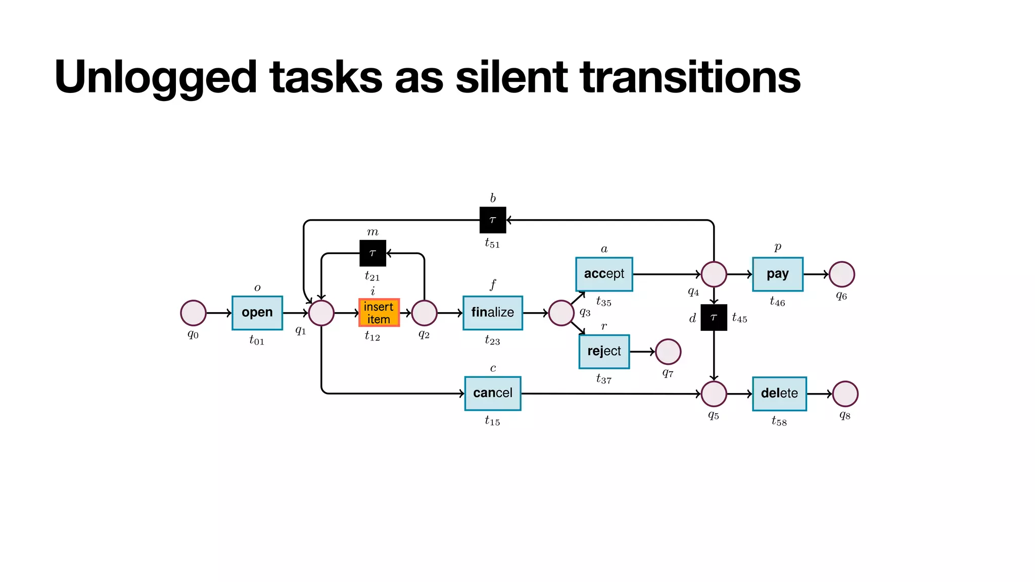
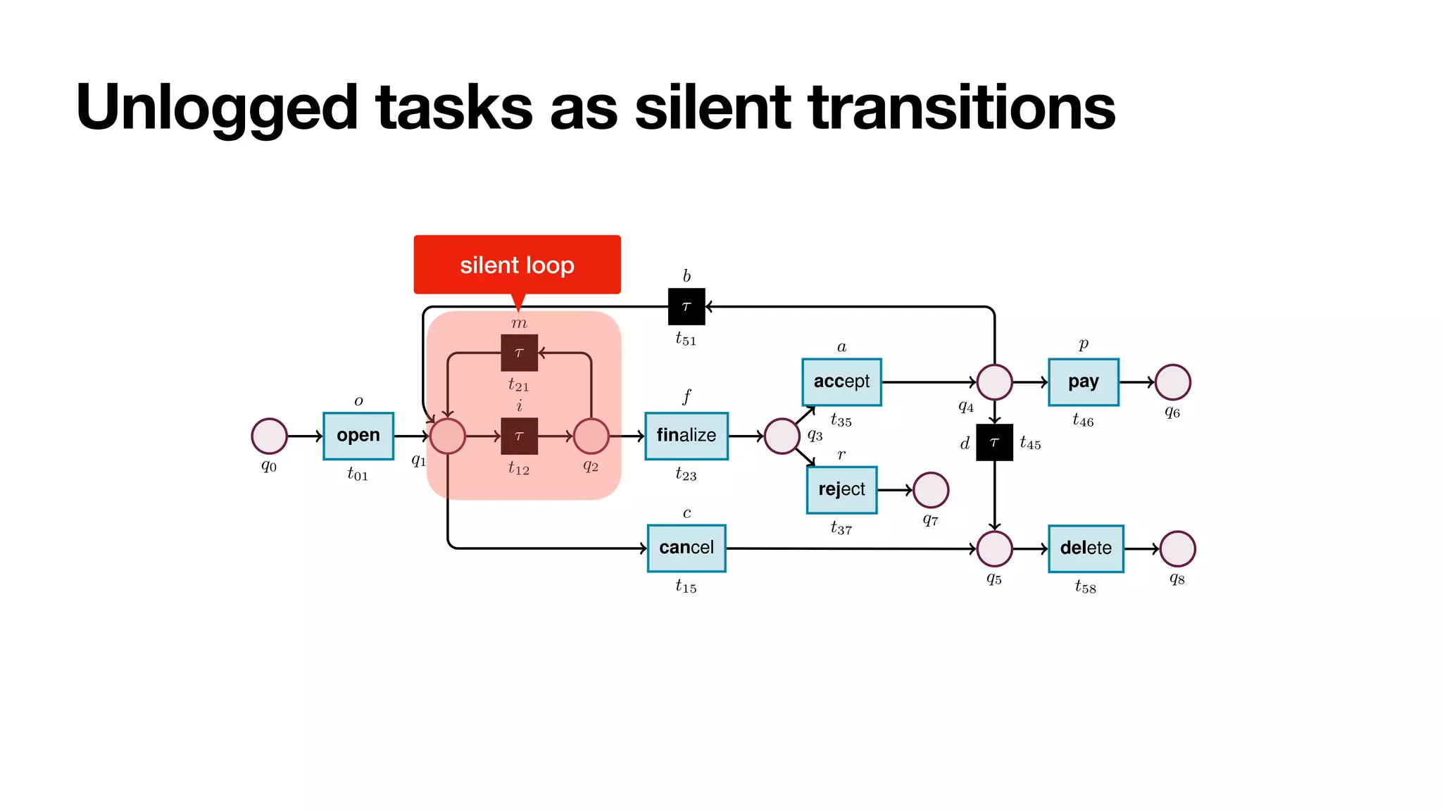
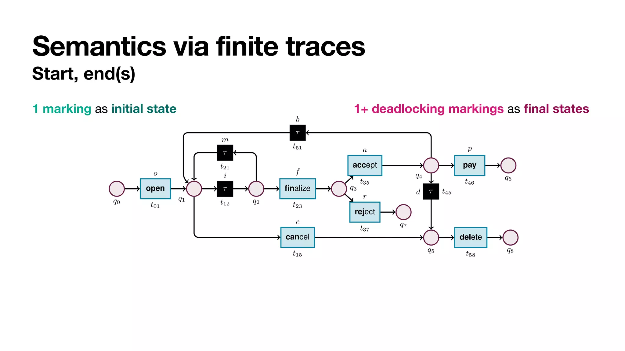
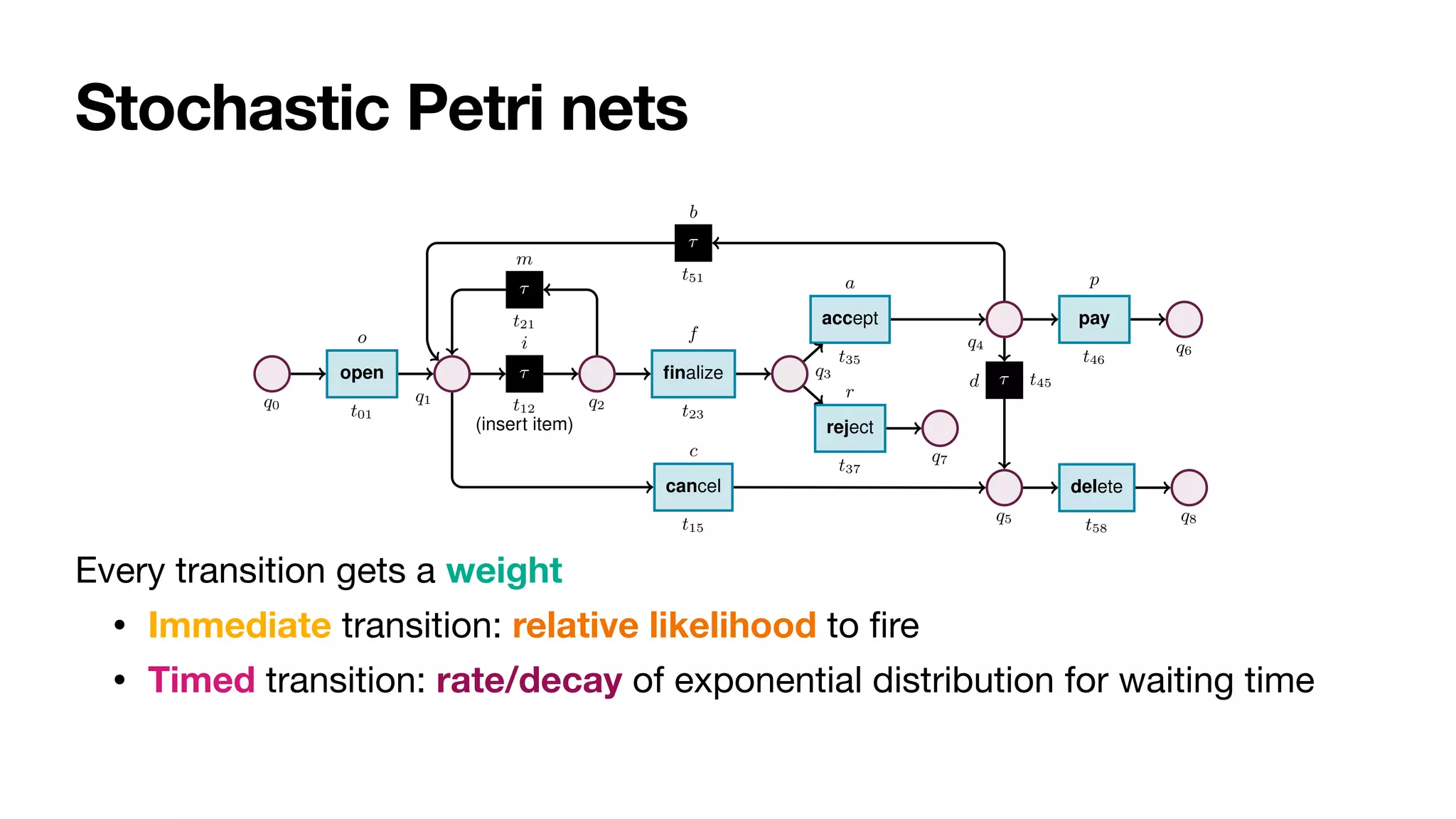
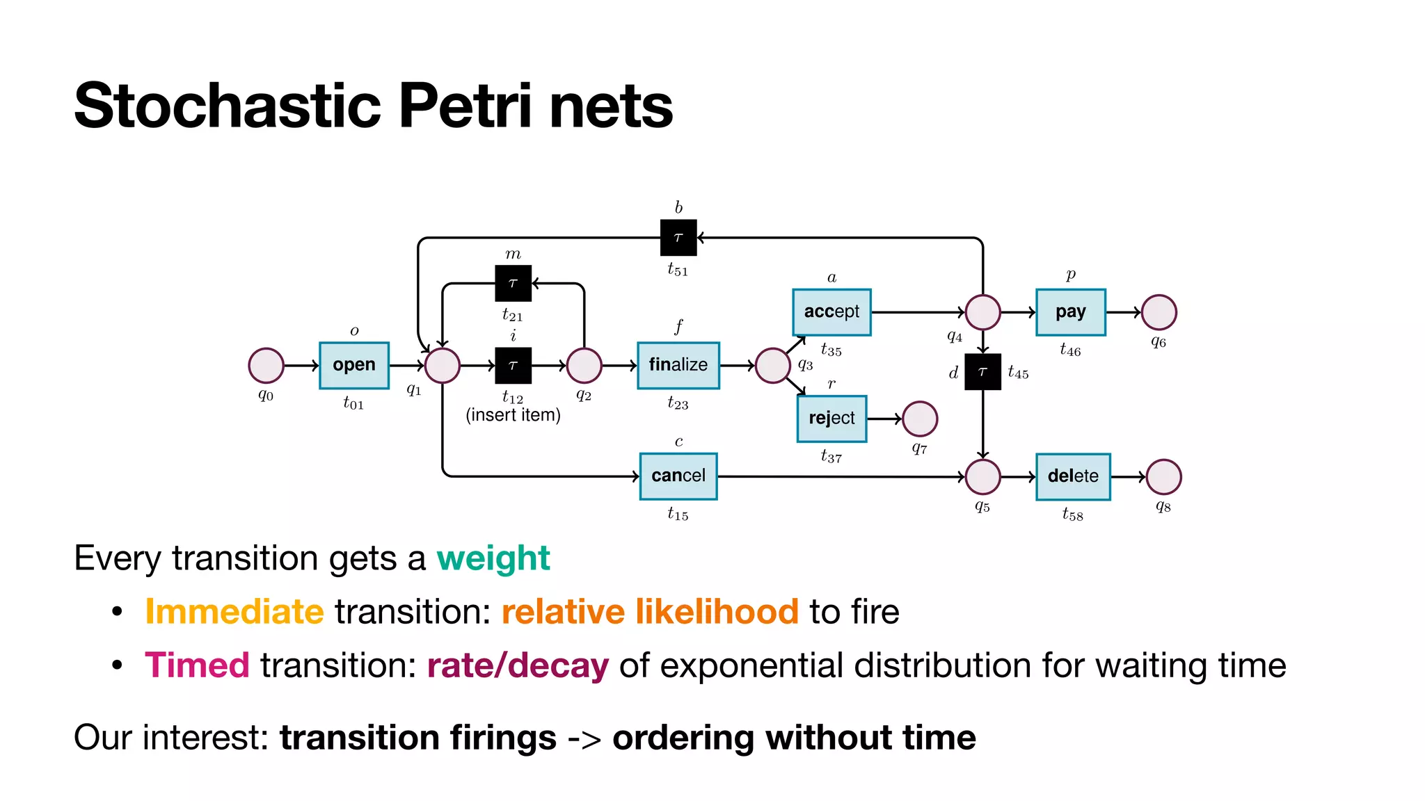
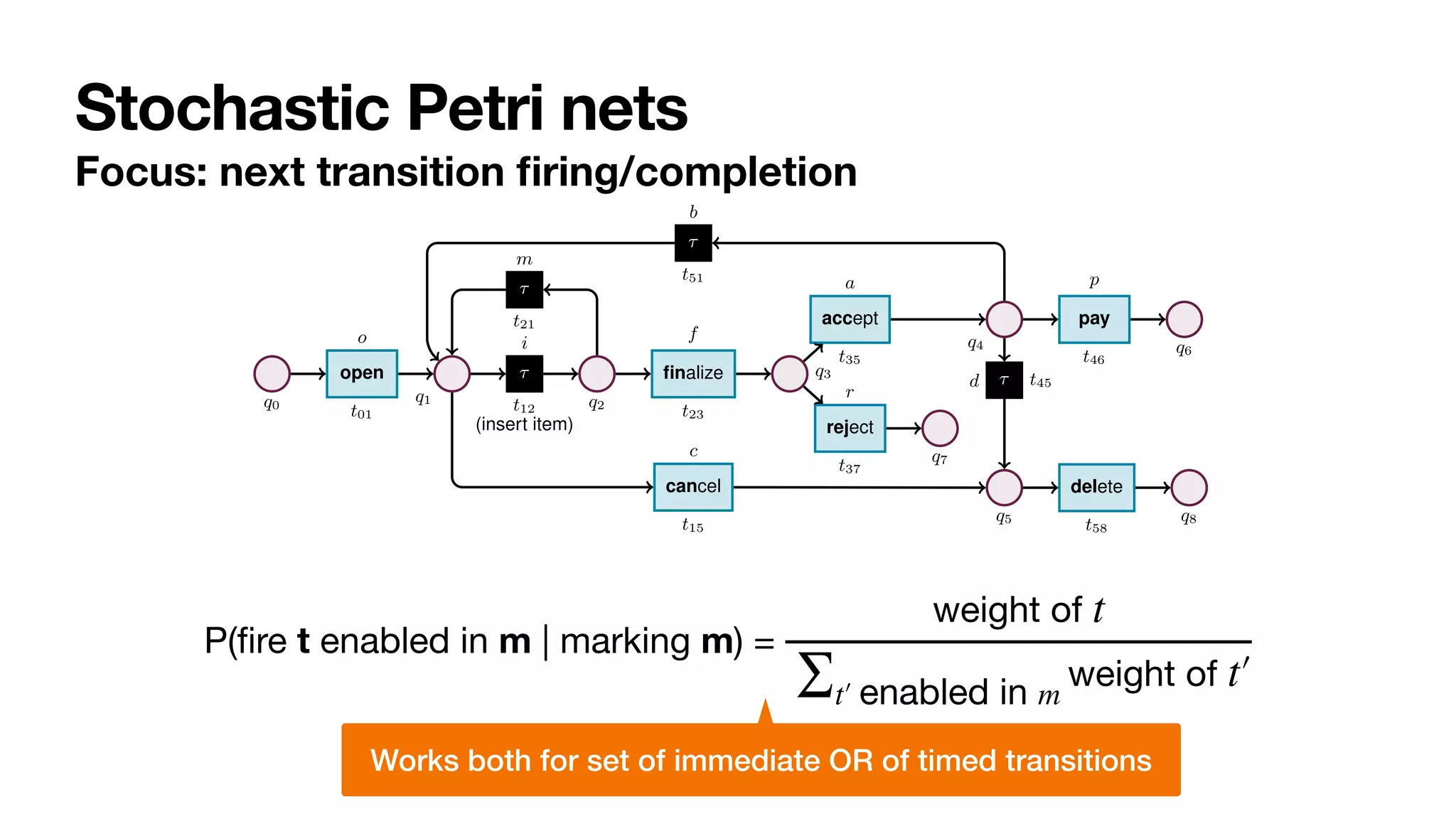
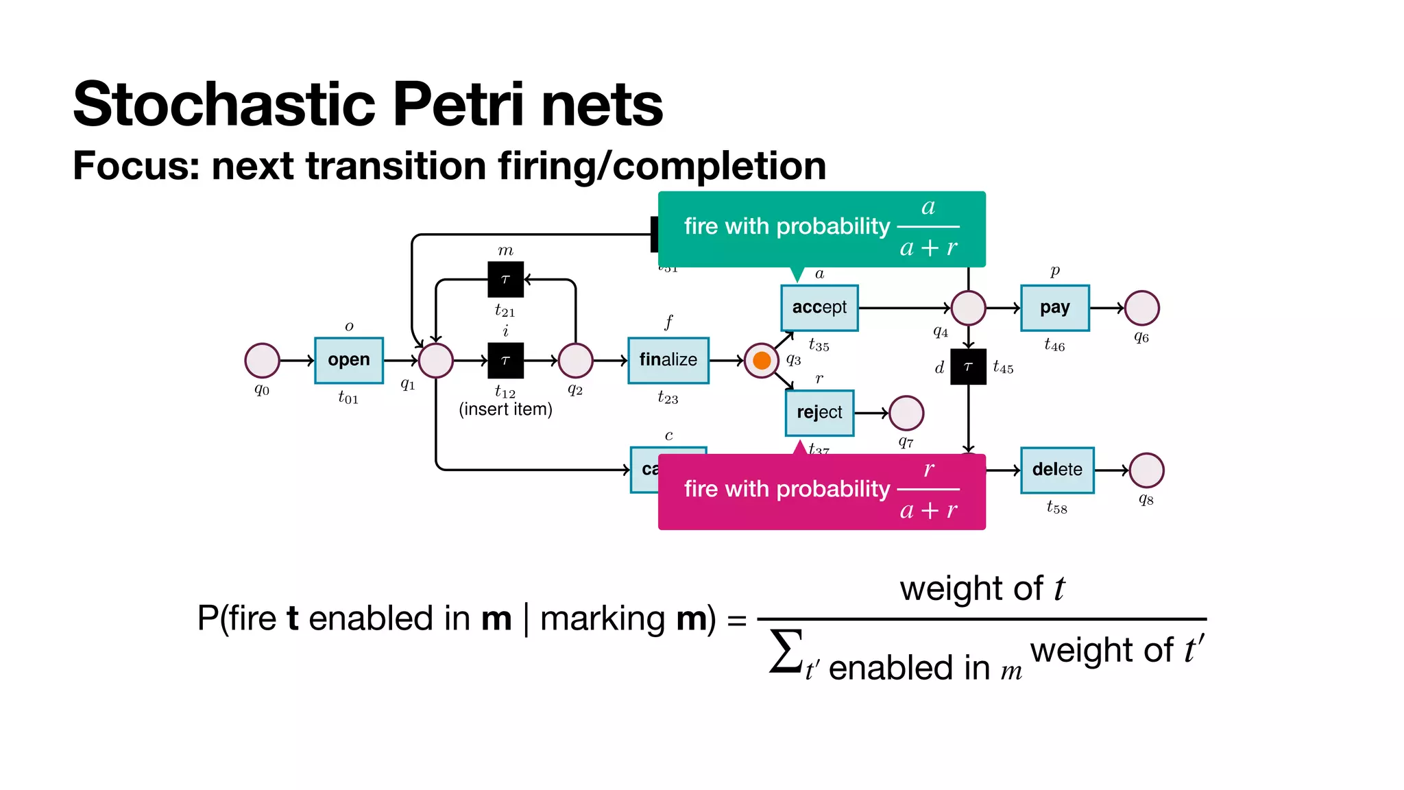
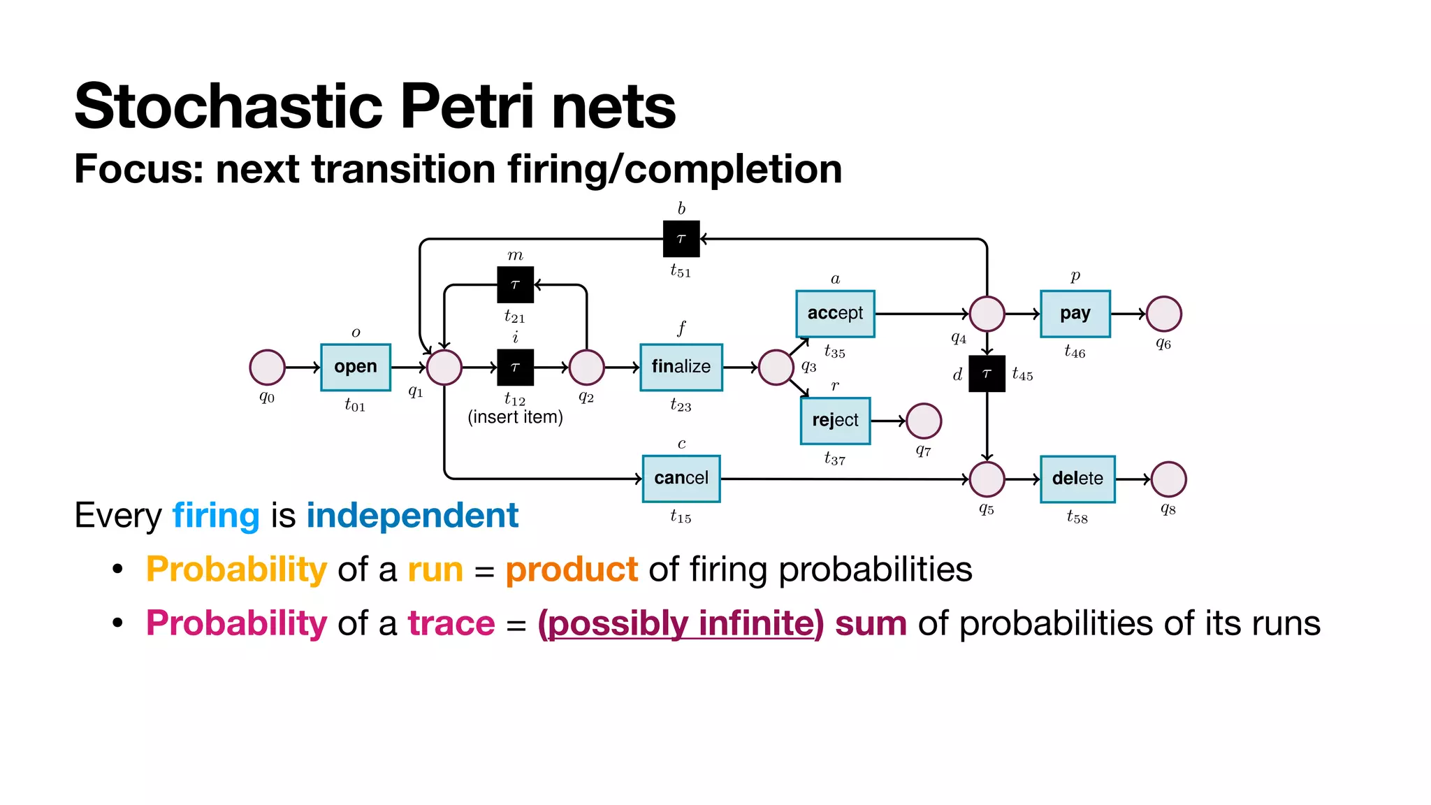
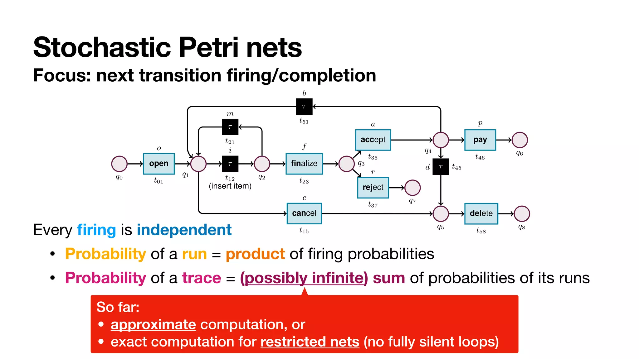
Fig. 2: Stochastic net of an order-to-cash process. Weights are presented symbolically.
Transition t12 captures a task that cannot be logged, and so is modelled as silent.
Definition 1 (Labelled Petri net). A labelled Petri net N is a tuple hQ, T, F, `i, where:
(i) Q is a finite set of places; (ii) T is a finite set of transitions, disjoint from Q (i.e.,
Q T = ;); (iii) F ✓ (Q ⇥ T) [ (T ⇥ Q) is a flow relation connecting places to
1 marking as initial state 1+ deadlock markings as
fi
nal states
initial state
[q0]
fi
nal “paid” state
[q6]
fi
nal “deleted” state
[q8]
fi
nal “rejected” state
[q7]](https://image.slidesharecdn.com/bpm2022-stochastic-reasoning-220922205316-6b26f0e0/75/Reasoning-on-Labelled-Petri-Nets-and-Their-Dynamics-in-a-Stochastic-Setting-15-2048.jpg)
![Semantics via finite traces
Runs and traces
4 Sander J.J. Leemans et al.
q0
open
t01
o
q1
⌧
t12
i
(insert item)
q2
⌧
t21
m
finalize
t23
f
q3
reject
t37
r
q7
accept
t35
a
q4
⌧
t51
b
pay
t46
p
q6
⌧ t45
d
q5
cancel
t15
c
delete
t58
q8
Fig. 2: Stochastic net of an order-to-cash process. Weights are presented symbolically.
Transition t12 captures a task that cannot be logged, and so is modelled as silent.
Definition 1 (Labelled Petri net). A labelled Petri net N is a tuple hQ, T, F, `i, where:
(i) Q is a finite set of places; (ii) T is a finite set of transitions, disjoint from Q (i.e.,
Q T = ;); (iii) F ✓ (Q ⇥ T) [ (T ⇥ Q) is a flow relation connecting places to
1 marking as initial state 1+ deadlock markings as
fi
nal states
initial state
[q0]
Run: valid sequence of transitions from the initial state to some
fi
nal state
Trace: projection of the run on labels of visible transitions
How many runs for the same trace?
Potentially in
fi
nitely many!
fi
nal “paid” state
[q6]
fi
nal “deleted” state
[q8]
fi
nal “rejected” state
[q7]](https://image.slidesharecdn.com/bpm2022-stochastic-reasoning-220922205316-6b26f0e0/75/Reasoning-on-Labelled-Petri-Nets-and-Their-Dynamics-in-a-Stochastic-Setting-16-2048.jpg)
![Semantics via finite traces
Runs and traces
4 Sander J.J. Leemans et al.
q0
open
t01
o
q1
⌧
t12
i
(insert item)
q2
⌧
t21
m
finalize
t23
f
q3
reject
t37
r
q7
accept
t35
a
q4
⌧
t51
b
pay
t46
p
q6
⌧ t45
d
q5
cancel
t15
c
delete
t58
q8
Fig. 2: Stochastic net of an order-to-cash process. Weights are presented symbolically.
Transition t12 captures a task that cannot be logged, and so is modelled as silent.
Definition 1 (Labelled Petri net). A labelled Petri net N is a tuple hQ, T, F, `i, where:
(i) Q is a finite set of places; (ii) T is a finite set of transitions, disjoint from Q (i.e.,
Q T = ;); (iii) F ✓ (Q ⇥ T) [ (T ⇥ Q) is a flow relation connecting places to
1 marking as initial state 1+ deadlock markings as
fi
nal states
initial state
[q0]
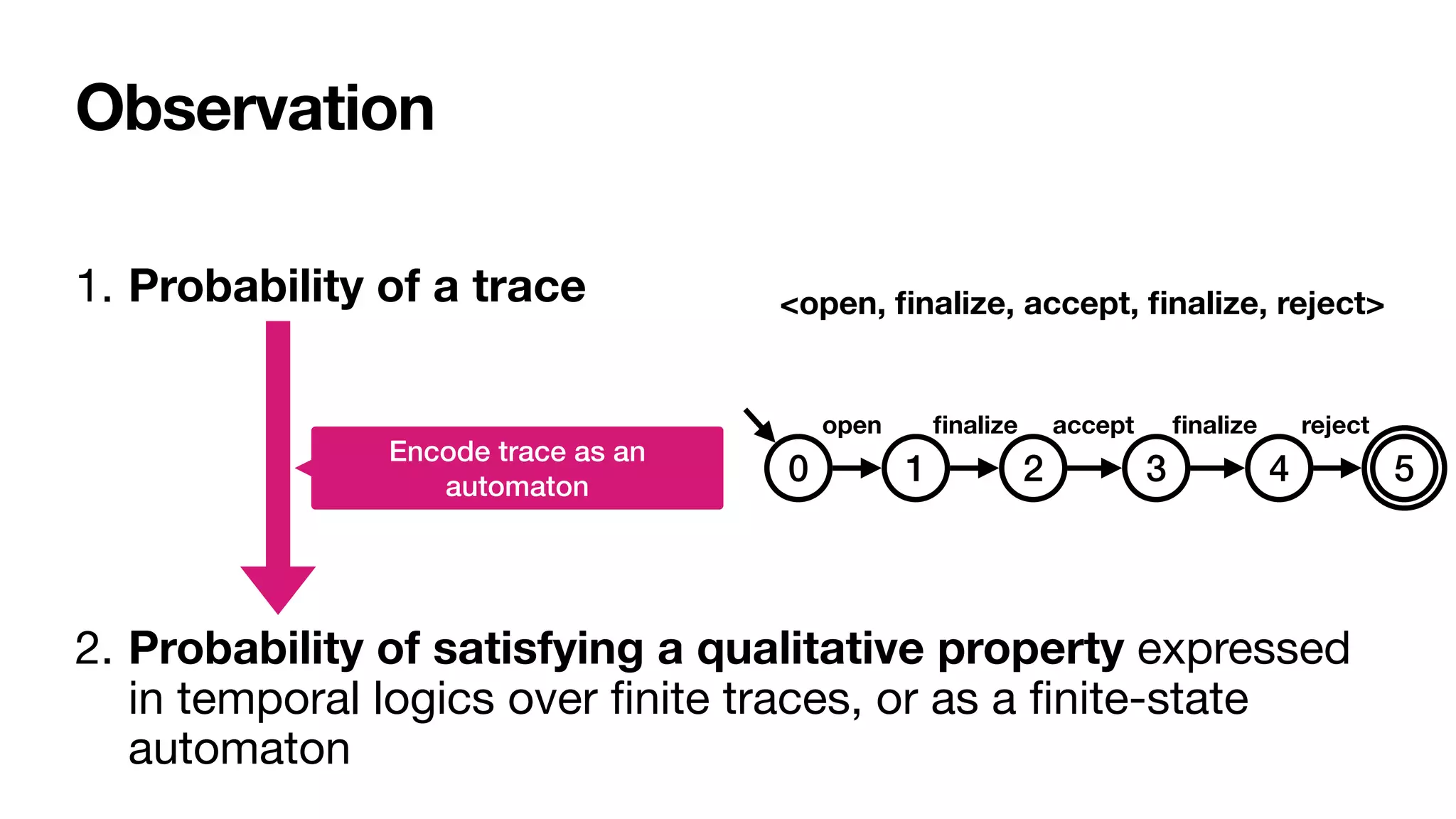
<open,
fi
nalize, accept,
fi
nalize, reject>
fi
nal “paid” state
[q6]
fi
nal “deleted” state
[q8]
fi
nal “rejected” state
[q7]](https://image.slidesharecdn.com/bpm2022-stochastic-reasoning-220922205316-6b26f0e0/75/Reasoning-on-Labelled-Petri-Nets-and-Their-Dynamics-in-a-Stochastic-Setting-17-2048.jpg)
![Semantics via finite traces
Runs and traces
4 Sander J.J. Leemans et al.
q0
open
t01
o
q1
⌧
t12
i
(insert item)
q2
⌧
t21
m
finalize
t23
f
q3
reject
t37
r
q7
accept
t35
a
q4
⌧
t51
b
pay
t46
p
q6
⌧ t45
d
q5
cancel
t15
c
delete
t58
q8
Fig. 2: Stochastic net of an order-to-cash process. Weights are presented symbolically.
Transition t12 captures a task that cannot be logged, and so is modelled as silent.
Definition 1 (Labelled Petri net). A labelled Petri net N is a tuple hQ, T, F, `i, where:
(i) Q is a finite set of places; (ii) T is a finite set of transitions, disjoint from Q (i.e.,
Q T = ;); (iii) F ✓ (Q ⇥ T) [ (T ⇥ Q) is a flow relation connecting places to
1 marking as initial state 1+ deadlock markings as
fi
nal states
initial state
[q0]
fi
nal “paid” state
[q6]
fi
nal “deleted” state
[q8]
<open,
fi
nalize, accept,
fi
nalize, reject>
fi
nal “rejected” state
[q7]](https://image.slidesharecdn.com/bpm2022-stochastic-reasoning-220922205316-6b26f0e0/75/Reasoning-on-Labelled-Petri-Nets-and-Their-Dynamics-in-a-Stochastic-Setting-18-2048.jpg)
![From net to transition system
4 Sander J.J. Leemans et al.
q0
open
t01
o
q1
⌧
t12
i
(insert item)
q2
⌧
t21
m
finalize
t23
f
q3
reject
t37
r
q7
accept
t35
a
q4
⌧
t51
b
pay
t46
p
q6
⌧ t45
d
q5
cancel
t15
c
delete
t58
q8
Fig. 2: Stochastic net of an order-to-cash process. Weights are presented symbolically.
Transition t12 captures a task that cannot be logged, and so is modelled as silent.
Definition 1 (Labelled Petri net). A labelled Petri net N is a tuple hQ, T, F, `i, where:
(i) Q is a finite set of places; (ii) T is a finite set of transitions, disjoint from Q (i.e.,
Q T = ;); (iii) F ✓ (Q ⇥ T) [ (T ⇥ Q) is a flow relation connecting places to
transitions and transitions to places; (iv) ` : T ! ⌃ is a labelling function mapping
each transition t 2 T to a corresponding label `(t) that is either a task name from ⌃ of
initial state
[q0]
fi
nal “paid” state
[q6]
fi
nal “deleted” state
[q8]
fi
nal “rejected” state
[q7]
6 Sander J.J. Leemans et al.
s0
[q0]
s1
[q1]
s2
[q2]
s3
[q3]
s4
[q4]
s7
[q7]
s5
[q5]
s6
[q6]
s8
[q8]
1
open
⇢i = i
i+c
⌧
⇢m = m
m+f
⌧
⇢f = f
m+f
fin ⇢a
=
a
a+r
acc
⇢r = r
a+r
rej
⇢b = b
b+p+d
⌧
⇢c = c
i+c can
⇢d = d
b+p+d
⌧
⇢p = d
b+p+d
pay
1
del](https://image.slidesharecdn.com/bpm2022-stochastic-reasoning-220922205316-6b26f0e0/75/Reasoning-on-Labelled-Petri-Nets-and-Their-Dynamics-in-a-Stochastic-Setting-19-2048.jpg)
![Semantics via stochastic transition systems
4 Sander J.J. Leemans et al.
q0
open
t01
o
q1
⌧
t12
i
(insert item)
q2
⌧
t21
m
finalize
t23
f
q3
reject
t37
r
q7
accept
t35
a
q4
⌧
t51
b
pay
t46
p
q6
⌧ t45
d
q5
cancel
t15
c
delete
t58
q8
Fig. 2: Stochastic net of an order-to-cash process. Weights are presented symbolically.
Transition t12 captures a task that cannot be logged, and so is modelled as silent.
Definition 1 (Labelled Petri net). A labelled Petri net N is a tuple hQ, T, F, `i, where:
(i) Q is a finite set of places; (ii) T is a finite set of transitions, disjoint from Q (i.e.,
Q T = ;); (iii) F ✓ (Q ⇥ T) [ (T ⇥ Q) is a flow relation connecting places to
transitions and transitions to places; (iv) ` : T ! ⌃ is a labelling function mapping
each transition t 2 T to a corresponding label `(t) that is either a task name from ⌃ of
initial state
[q0]
fi
nal “paid” state
[q6]
fi
nal “deleted” state
[q8]
fi
nal “rejected” state
[q7]
6 Sander J.J. Leemans et al.
s0
[q0]
s1
[q1]
s2
[q2]
s3
[q3]
s4
[q4]
s7
[q7]
s5
[q5]
s6
[q6]
s8
[q8]
1
open
⇢i = i
i+c
⌧
⇢m = m
m+f
⌧
⇢f = f
m+f
fin ⇢a
=
a
a+r
acc
⇢r = r
a+r
rej
⇢b = b
b+p+d
⌧
⇢c = c
i+c can
⇢d = d
b+p+d
⌧
⇢p = d
b+p+d
pay
1
del
Looks familiar?](https://image.slidesharecdn.com/bpm2022-stochastic-reasoning-220922205316-6b26f0e0/75/Reasoning-on-Labelled-Petri-Nets-and-Their-Dynamics-in-a-Stochastic-Setting-26-2048.jpg)


![Outcome probability
What is the probability of ending with order paid?
6 Sander J.J. Leemans et al.
s0
[q0]
s1
[q1]
s2
[q2]
s3
[q3]
s4
[q4]
s7
[q7]
s5
[q5]
s6
[q6]
s8
[q8]
1
open
⇢i = i
i+c
⌧
⇢m = m
m+f
⌧
⇢f = f
m+f
fin ⇢a
=
a
a+r
acc
⇢r = r
a+r
rej
⇢b = b
b+p+d
⌧
⇢c = c
i+c can
⇢d = d
b+p+d
⌧
⇢p = d
b+p+d
pay
1
del
Fig. 3: Stochastic reachability graph of the order-to-cash bounded stochastic PNP.
States are named. The initial state is shown with a small incoming edge. Final states
have a double countour.](https://image.slidesharecdn.com/bpm2022-stochastic-reasoning-220922205316-6b26f0e0/75/Reasoning-on-Labelled-Petri-Nets-and-Their-Dynamics-in-a-Stochastic-Setting-35-2048.jpg)
![Outcome probability
What is the probability of ending with order paid?
What matters: progression from state to state -> Markov chain
6 Sander J.J. Leemans et al.
s0
[q0]
s1
[q1]
s2
[q2]
s3
[q3]
s4
[q4]
s7
[q7]
s5
[q5]
s6
[q6]
s8
[q8]
1
open
⇢i = i
i+c
⌧
⇢m = m
m+f
⌧
⇢f = f
m+f
fin ⇢a
=
a
a+r
acc
⇢r = r
a+r
rej
⇢b = b
b+p+d
⌧
⇢c = c
i+c can
⇢d = d
b+p+d
⌧
⇢p = d
b+p+d
pay
1
del
Fig. 3: Stochastic reachability graph of the order-to-cash bounded stochastic PNP.
States are named. The initial state is shown with a small incoming edge. Final states
have a double countour.](https://image.slidesharecdn.com/bpm2022-stochastic-reasoning-220922205316-6b26f0e0/75/Reasoning-on-Labelled-Petri-Nets-and-Their-Dynamics-in-a-Stochastic-Setting-36-2048.jpg)
![Outcome probability
What is the probability of ending with order paid?
Each state -> variable for probability of reaching the desired one from there
3 cases:
•
fi
nal desired state (good deadlock)
•
fi
nal non-desired state (bad deadlock)
• other states…
6 Sander J.J. Leemans et al.
s0
[q0]
s1
[q1]
s2
[q2]
s3
[q3]
s4
[q4]
s7
[q7]
s5
[q5]
s6
[q6]
s8
[q8]
1
open
⇢i = i
i+c
⌧
⇢m = m
m+f
⌧
⇢f = f
m+f
fin ⇢a
=
a
a+r
acc
⇢r = r
a+r
rej
⇢b = b
b+p+d
⌧
⇢c = c
i+c can
⇢d = d
b+p+d
⌧
⇢p = d
b+p+d
pay
1
del
Fig. 3: Stochastic reachability graph of the order-to-cash bounded stochastic PNP.
States are named. The initial state is shown with a small incoming edge. Final states
have a double countour.](https://image.slidesharecdn.com/bpm2022-stochastic-reasoning-220922205316-6b26f0e0/75/Reasoning-on-Labelled-Petri-Nets-and-Their-Dynamics-in-a-Stochastic-Setting-37-2048.jpg)
![Outcome probability
What is the probability of ending with order paid?
Each state -> variable for probability of reaching the desired one from there
3 cases:
•
fi
nal desired state (good deadlock) -> 1
•
fi
nal non-desired state (bad deadlock) -> 0
• other states… -> recursive de
fi
nition via linear equations
6 Sander J.J. Leemans et al.
s0
[q0]
s1
[q1]
s2
[q2]
s3
[q3]
s4
[q4]
s7
[q7]
s5
[q5]
s6
[q6]
s8
[q8]
1
open
⇢i = i
i+c
⌧
⇢m = m
m+f
⌧
⇢f = f
m+f
fin ⇢a
=
a
a+r
acc
⇢r = r
a+r
rej
⇢b = b
b+p+d
⌧
⇢c = c
i+c can
⇢d = d
b+p+d
⌧
⇢p = d
b+p+d
pay
1
del
Fig. 3: Stochastic reachability graph of the order-to-cash bounded stochastic PNP.
States are named. The initial state is shown with a small incoming edge. Final states
have a double countour.
x6 = 1
x8 = 0
x1 = ρix2 + ρcx5](https://image.slidesharecdn.com/bpm2022-stochastic-reasoning-220922205316-6b26f0e0/75/Reasoning-on-Labelled-Petri-Nets-and-Their-Dynamics-in-a-Stochastic-Setting-38-2048.jpg)
![Outcome probability
What is the probability of ending with order paid?
Each state -> variable for probability of reaching the desired one from there
3 cases:
•
fi
nal desired state (good deadlock) -> 1
•
fi
nal non-desired state (bad deadlock) -> 0
• other states… -> recursive de
fi
nition via linear equations
6 Sander J.J. Leemans et al.
s0
[q0]
s1
[q1]
s2
[q2]
s3
[q3]
s4
[q4]
s7
[q7]
s5
[q5]
s6
[q6]
s8
[q8]
1
open
⇢i = i
i+c
⌧
⇢m = m
m+f
⌧
⇢f = f
m+f
fin ⇢a
=
a
a+r
acc
⇢r = r
a+r
rej
⇢b = b
b+p+d
⌧
⇢c = c
i+c can
⇢d = d
b+p+d
⌧
⇢p = d
b+p+d
pay
1
del
Fig. 3: Stochastic reachability graph of the order-to-cash bounded stochastic PNP.
States are named. The initial state is shown with a small incoming edge. Final states
have a double countour.
} Solve for initial state variable!
x6 = 1
x8 = 0
x1 = ρix2 + ρcx5](https://image.slidesharecdn.com/bpm2022-stochastic-reasoning-220922205316-6b26f0e0/75/Reasoning-on-Labelled-Petri-Nets-and-Their-Dynamics-in-a-Stochastic-Setting-39-2048.jpg)
![Outcome probability
What is the probability of ending with order paid?
6 Sander J.J. Leemans et al.
s0
[q0]
s1
[q1]
s2
[q2]
s3
[q3]
s4
[q4]
s7
[q7]
s5
[q5]
s6
[q6]
s8
[q8]
1
open
⇢i = i
i+c
⌧
⇢m = m
m+f
⌧
⇢f = f
m+f
fin ⇢a
=
a
a+r
acc
⇢r = r
a+r
rej
⇢b = b
b+p+d
⌧
⇢c = c
i+c can
⇢d = d
b+p+d
⌧
⇢p = d
b+p+d
pay
1
del
Fig. 3: Stochastic reachability graph of the order-to-cash bounded stochastic PNP.
States are named. The initial state is shown with a small incoming edge. Final states
have a double countour.
marking [q0] and final marking [q1]. States s2 and s3 are livelock markings.
By recalling that states of RG(N) are markings of N, the schema (1) of equations
deals with final (deadlock) states, that in (1) with non-final deadlock states, and that in
(1) with non-final, non-deadlock states.
EF
N has always at least a solution. However, it may be indeterminate and thus admit
infinitely many ones, requiring in that case to pick the least committing (i.e., minimal
non-negative) solution. The latter case happens when N contains livelock markings.
This is illustrated in the following examples.
Example 2. Consider bounded stochastic PNP Norder (Figure 2). We want to solve the
problem OUTCOME-PROB(Norder, [q6]), to compute the probability that a created order
eventually completes the process by being paid. To do so, we solve E
[q6]
Norder
by encoding
the reachability graph of Figure 3 into:
xs8
= 0 xs5
= xs8
xs2
= ⇢mxs1
+ ⇢f xs3
xs7
= 0 xs4
= ⇢bxs1
+ ⇢dxs5
+ ⇢pxs6
xs1
= ⇢ixs2
+ ⇢cxs5
xs6
= 1 xs3
= ⇢axs4
+ ⇢rxs7
xs0
= xs1](https://image.slidesharecdn.com/bpm2022-stochastic-reasoning-220922205316-6b26f0e0/75/Reasoning-on-Labelled-Petri-Nets-and-Their-Dynamics-in-a-Stochastic-Setting-40-2048.jpg)
![marking [q0] and final marking [q1]. States s2 and s3 are livelock markings.
By recalling that states of RG(N) are markings of N, the schema (1) of equations
deals with final (deadlock) states, that in (1) with non-final deadlock states, and that in
(1) with non-final, non-deadlock states.
EF
N has always at least a solution. However, it may be indeterminate and thus admit
infinitely many ones, requiring in that case to pick the least committing (i.e., minimal
non-negative) solution. The latter case happens when N contains livelock markings.
This is illustrated in the following examples.
Example 2. Consider bounded stochastic PNP Norder (Figure 2). We want to solve the
problem OUTCOME-PROB(Norder, [q6]), to compute the probability that a created order
eventually completes the process by being paid. To do so, we solve E
[q6]
Norder
by encoding
the reachability graph of Figure 3 into:
xs8
= 0 xs5
= xs8
xs2
= ⇢mxs1
+ ⇢f xs3
xs7
= 0 xs4
= ⇢bxs1
+ ⇢dxs5
+ ⇢pxs6
xs1
= ⇢ixs2
+ ⇢cxs5
xs6
= 1 xs3
= ⇢axs4
+ ⇢rxs7
xs0
= xs1
Outcome probability
What is the probability of ending with order paid?
6 Sander J.J. Leemans et al.
s0
[q0]
s1
[q1]
s2
[q2]
s3
[q3]
s4
[q4]
s7
[q7]
s5
[q5]
s6
[q6]
s8
[q8]
1
open
⇢i = i
i+c
⌧
⇢m = m
m+f
⌧
⇢f = f
m+f
fin ⇢a
=
a
a+r
acc
⇢r = r
a+r
rej
⇢b = b
b+p+d
⌧
⇢c = c
i+c can
⇢d = d
b+p+d
⌧
⇢p = d
b+p+d
pay
1
del
Fig. 3: Stochastic reachability graph of the order-to-cash bounded stochastic PNP.
States are named. The initial state is shown with a small incoming edge. Final states
have a double countour.
}
x0 =
ρiρf ρaρp
1 − ρiρm − ρiρf ρaρb](https://image.slidesharecdn.com/bpm2022-stochastic-reasoning-220922205316-6b26f0e0/75/Reasoning-on-Labelled-Petri-Nets-and-Their-Dynamics-in-a-Stochastic-Setting-41-2048.jpg)
![marking [q0] and final marking [q1]. States s2 and s3 are livelock markings.
By recalling that states of RG(N) are markings of N, the schema (1) of equations
deals with final (deadlock) states, that in (1) with non-final deadlock states, and that in
(1) with non-final, non-deadlock states.
EF
N has always at least a solution. However, it may be indeterminate and thus admit
infinitely many ones, requiring in that case to pick the least committing (i.e., minimal
non-negative) solution. The latter case happens when N contains livelock markings.
This is illustrated in the following examples.
Example 2. Consider bounded stochastic PNP Norder (Figure 2). We want to solve the
problem OUTCOME-PROB(Norder, [q6]), to compute the probability that a created order
eventually completes the process by being paid. To do so, we solve E
[q6]
Norder
by encoding
the reachability graph of Figure 3 into:
xs8
= 0 xs5
= xs8
xs2
= ⇢mxs1
+ ⇢f xs3
xs7
= 0 xs4
= ⇢bxs1
+ ⇢dxs5
+ ⇢pxs6
xs1
= ⇢ixs2
+ ⇢cxs5
xs6
= 1 xs3
= ⇢axs4
+ ⇢rxs7
xs0
= xs1
Outcome probability
What is the probability of ending with order paid?
6 Sander J.J. Leemans et al.
s0
[q0]
s1
[q1]
s2
[q2]
s3
[q3]
s4
[q4]
s7
[q7]
s5
[q5]
s6
[q6]
s8
[q8]
1
open
⇢i = i
i+c
⌧
⇢m = m
m+f
⌧
⇢f = f
m+f
fin ⇢a
=
a
a+r
acc
⇢r = r
a+r
rej
⇢b = b
b+p+d
⌧
⇢c = c
i+c can
⇢d = d
b+p+d
⌧
⇢p = d
b+p+d
pay
1
del
Fig. 3: Stochastic reachability graph of the order-to-cash bounded stochastic PNP.
States are named. The initial state is shown with a small incoming edge. Final states
have a double countour.
}
x0 =
ρiρf ρaρp
1 − ρiρm − ρiρf ρaρb](https://image.slidesharecdn.com/bpm2022-stochastic-reasoning-220922205316-6b26f0e0/75/Reasoning-on-Labelled-Petri-Nets-and-Their-Dynamics-in-a-Stochastic-Setting-42-2048.jpg)
![marking [q0] and final marking [q1]. States s2 and s3 are livelock markings.
By recalling that states of RG(N) are markings of N, the schema (1) of equations
deals with final (deadlock) states, that in (1) with non-final deadlock states, and that in
(1) with non-final, non-deadlock states.
EF
N has always at least a solution. However, it may be indeterminate and thus admit
infinitely many ones, requiring in that case to pick the least committing (i.e., minimal
non-negative) solution. The latter case happens when N contains livelock markings.
This is illustrated in the following examples.
Example 2. Consider bounded stochastic PNP Norder (Figure 2). We want to solve the
problem OUTCOME-PROB(Norder, [q6]), to compute the probability that a created order
eventually completes the process by being paid. To do so, we solve E
[q6]
Norder
by encoding
the reachability graph of Figure 3 into:
xs8
= 0 xs5
= xs8
xs2
= ⇢mxs1
+ ⇢f xs3
xs7
= 0 xs4
= ⇢bxs1
+ ⇢dxs5
+ ⇢pxs6
xs1
= ⇢ixs2
+ ⇢cxs5
xs6
= 1 xs3
= ⇢axs4
+ ⇢rxs7
xs0
= xs1
Outcome probability
What is the probability of ending with order paid?
6 Sander J.J. Leemans et al.
s0
[q0]
s1
[q1]
s2
[q2]
s3
[q3]
s4
[q4]
s7
[q7]
s5
[q5]
s6
[q6]
s8
[q8]
1
open
⇢i = i
i+c
⌧
⇢m = m
m+f
⌧
⇢f = f
m+f
fin ⇢a
=
a
a+r
acc
⇢r = r
a+r
rej
⇢b = b
b+p+d
⌧
⇢c = c
i+c can
⇢d = d
b+p+d
⌧
⇢p = d
b+p+d
pay
1
del
Fig. 3: Stochastic reachability graph of the order-to-cash bounded stochastic PNP.
States are named. The initial state is shown with a small incoming edge. Final states
have a double countour.
}
x0 =
ρiρf ρaρp
1 − ρiρm − ρiρf ρaρb](https://image.slidesharecdn.com/bpm2022-stochastic-reasoning-220922205316-6b26f0e0/75/Reasoning-on-Labelled-Petri-Nets-and-Their-Dynamics-in-a-Stochastic-Setting-43-2048.jpg)
![marking [q0] and final marking [q1]. States s2 and s3 are livelock markings.
By recalling that states of RG(N) are markings of N, the schema (1) of equations
deals with final (deadlock) states, that in (1) with non-final deadlock states, and that in
(1) with non-final, non-deadlock states.
EF
N has always at least a solution. However, it may be indeterminate and thus admit
infinitely many ones, requiring in that case to pick the least committing (i.e., minimal
non-negative) solution. The latter case happens when N contains livelock markings.
This is illustrated in the following examples.
Example 2. Consider bounded stochastic PNP Norder (Figure 2). We want to solve the
problem OUTCOME-PROB(Norder, [q6]), to compute the probability that a created order
eventually completes the process by being paid. To do so, we solve E
[q6]
Norder
by encoding
the reachability graph of Figure 3 into:
xs8
= 0 xs5
= xs8
xs2
= ⇢mxs1
+ ⇢f xs3
xs7
= 0 xs4
= ⇢bxs1
+ ⇢dxs5
+ ⇢pxs6
xs1
= ⇢ixs2
+ ⇢cxs5
xs6
= 1 xs3
= ⇢axs4
+ ⇢rxs7
xs0
= xs1
Outcome probability
What is the probability of ending with order paid?
6 Sander J.J. Leemans et al.
s0
[q0]
s1
[q1]
s2
[q2]
s3
[q3]
s4
[q4]
s7
[q7]
s5
[q5]
s6
[q6]
s8
[q8]
1
open
⇢i = i
i+c
⌧
⇢m = m
m+f
⌧
⇢f = f
m+f
fin ⇢a
=
a
a+r
acc
⇢r = r
a+r
rej
⇢b = b
b+p+d
⌧
⇢c = c
i+c can
⇢d = d
b+p+d
⌧
⇢p = d
b+p+d
pay
1
del
Fig. 3: Stochastic reachability graph of the order-to-cash bounded stochastic PNP.
States are named. The initial state is shown with a small incoming edge. Final states
have a double countour.
}
x0 =
ρiρf ρaρp
1 − ρiρm − ρiρf ρaρb](https://image.slidesharecdn.com/bpm2022-stochastic-reasoning-220922205316-6b26f0e0/75/Reasoning-on-Labelled-Petri-Nets-and-Their-Dynamics-in-a-Stochastic-Setting-44-2048.jpg)
![More care needed…
Reasoning on Labelled Petri Nets and their Dynamics in a Stochastic Setting 9
q0
a
t01
a
q1
b
t02
b
q2
c
t23
c
q3
d
t32
d
e t33
e
(a) Stochastic net.
s0
[q0]
s1
[q1]
s2
[q2]
s3
[q3]
a
⇢a
=
a
a+b
b
⇢b = b
a+b c
d
⇢d = d
d+e e
⇢e = e
e+d
(b) Reachability graph.
Fig. 4: Reachability graph (b) of a bounded stochastic PNP with net shown in (a), initial
initial state
[q0]
fi
nal state
[q1]](https://image.slidesharecdn.com/bpm2022-stochastic-reasoning-220922205316-6b26f0e0/75/Reasoning-on-Labelled-Petri-Nets-and-Their-Dynamics-in-a-Stochastic-Setting-45-2048.jpg)
![More care needed…
Reasoning on Labelled Petri Nets and their Dynamics in a Stochastic Setting 9
q0
a
t01
a
q1
b
t02
b
q2
c
t23
c
q3
d
t32
d
e t33
e
(a) Stochastic net.
s0
[q0]
s1
[q1]
s2
[q2]
s3
[q3]
a
⇢a
=
a
a+b
b
⇢b = b
a+b c
d
⇢d = d
d+e e
⇢e = e
e+d
(b) Reachability graph.
Fig. 4: Reachability graph (b) of a bounded stochastic PNP with net shown in (a), initial
initial state
[q0]
fi
nal state
[q1]
livelock](https://image.slidesharecdn.com/bpm2022-stochastic-reasoning-220922205316-6b26f0e0/75/Reasoning-on-Labelled-Petri-Nets-and-Their-Dynamics-in-a-Stochastic-Setting-46-2048.jpg)
![More care needed…
Reasoning on Labelled Petri Nets and their Dynamics in a Stochastic Setting 9
q0
a
t01
a
q1
b
t02
b
q2
c
t23
c
q3
d
t32
d
e t33
e
(a) Stochastic net.
s0
[q0]
s1
[q1]
s2
[q2]
s3
[q3]
a
⇢a
=
a
a+b
b
⇢b = b
a+b c
d
⇢d = d
d+e e
⇢e = e
e+d
(b) Reachability graph.
Fig. 4: Reachability graph (b) of a bounded stochastic PNP with net shown in (a), initial
initial state
[q0]
fi
nal state
[q1]
livelock x3 = 0
x2 = 0](https://image.slidesharecdn.com/bpm2022-stochastic-reasoning-220922205316-6b26f0e0/75/Reasoning-on-Labelled-Petri-Nets-and-Their-Dynamics-in-a-Stochastic-Setting-47-2048.jpg)
![Model checking
What are the traces of the net that satisfy my property?
6 Sander J.J. Leemans et al.
s0
[q0]
s1
[q1]
s2
[q2]
s3
[q3]
s4
[q4]
s7
[q7]
s5
[q5]
s6
[q6]
s8
[q8]
1
open
⇢i = i
i+c
⌧
⇢m = m
m+f
⌧
⇢f = f
m+f
fin ⇢a
=
a
a+r
acc
⇢r = r
a+r
rej
⇢b = b
b+p+d
⌧
⇢c = c
i+c can
⇢d = d
b+p+d
⌧
⇢p = d
b+p+d
pay
1
del
Fig. 3: Stochastic reachability graph of the order-to-cash bounded stochastic PNP.
States are named. The initial state is shown with a small incoming edge. Final states
have a double countour.
property: good,
fi
nite traces (via an automaton)](https://image.slidesharecdn.com/bpm2022-stochastic-reasoning-220922205316-6b26f0e0/75/Reasoning-on-Labelled-Petri-Nets-and-Their-Dynamics-in-a-Stochastic-Setting-51-2048.jpg)
![Model checking
What are the traces of the net that satisfy my property?
What matters: transitions and their labels -> transition system
6 Sander J.J. Leemans et al.
s0
[q0]
s1
[q1]
s2
[q2]
s3
[q3]
s4
[q4]
s7
[q7]
s5
[q5]
s6
[q6]
s8
[q8]
1
open
⇢i = i
i+c
⌧
⇢m = m
m+f
⌧
⇢f = f
m+f
fin ⇢a
=
a
a+r
acc
⇢r = r
a+r
rej
⇢b = b
b+p+d
⌧
⇢c = c
i+c can
⇢d = d
b+p+d
⌧
⇢p = d
b+p+d
pay
1
del
Fig. 3: Stochastic reachability graph of the order-to-cash bounded stochastic PNP.
States are named. The initial state is shown with a small incoming edge. Final states
have a double countour.
property: good,
fi
nite traces (via an automaton)](https://image.slidesharecdn.com/bpm2022-stochastic-reasoning-220922205316-6b26f0e0/75/Reasoning-on-Labelled-Petri-Nets-and-Their-Dynamics-in-a-Stochastic-Setting-52-2048.jpg)
![Automata-based product
6 Sander J.J. Leemans et al.
s0
[q0]
s1
[q1]
s2
[q2]
s3
[q3]
s4
[q4]
s7
[q7]
s5
[q5]
s6
[q6]
s8
[q8]
1
open
⇢i = i
i+c
⌧
⇢m = m
m+f
⌧
⇢f = f
m+f
fin ⇢a
=
a
a+r
acc
⇢r = r
a+r
rej
⇢b = b
b+p+d
⌧
⇢c = c
i+c can
⇢d = d
b+p+d
⌧
⇢p = d
b+p+d
pay
1
del
Fig. 3: Stochastic reachability graph of the order-to-cash bounded stochastic PNP.
States are named. The initial state is shown with a small incoming edge. Final states
have a double countour.
Definition 7 (Labelled transition system). A labelled transition system is a tuple
hS, s0, Sf , %i where: (i) S is a (possibly infinite) set of states; (ii) s0 2 S is the ini-
tial state; (iii) Sf ✓ S is the set of accepting states; (iv) % ✓ S ⇥⌃ ⇥ S is a⌃-labelled
transition relation. A run is a finite sequence of transitions leading from s0 to one of the
states in Sf in agreement with %. /
Due to our requirement that all final markings are deadlock markings, accepting states
0 1 2 3 4 5
open
fi
nalize accept
fi
nalize reject](https://image.slidesharecdn.com/bpm2022-stochastic-reasoning-220922205316-6b26f0e0/75/Reasoning-on-Labelled-Petri-Nets-and-Their-Dynamics-in-a-Stochastic-Setting-53-2048.jpg)
![Automata-based product
6 Sander J.J. Leemans et al.
s0
[q0]
s1
[q1]
s2
[q2]
s3
[q3]
s4
[q4]
s7
[q7]
s5
[q5]
s6
[q6]
s8
[q8]
1
open
⇢i = i
i+c
⌧
⇢m = m
m+f
⌧
⇢f = f
m+f
fin ⇢a
=
a
a+r
acc
⇢r = r
a+r
rej
⇢b = b
b+p+d
⌧
⇢c = c
i+c can
⇢d = d
b+p+d
⌧
⇢p = d
b+p+d
pay
1
del
Fig. 3: Stochastic reachability graph of the order-to-cash bounded stochastic PNP.
States are named. The initial state is shown with a small incoming edge. Final states
have a double countour.
Definition 7 (Labelled transition system). A labelled transition system is a tuple
hS, s0, Sf , %i where: (i) S is a (possibly infinite) set of states; (ii) s0 2 S is the ini-
tial state; (iii) Sf ✓ S is the set of accepting states; (iv) % ✓ S ⇥⌃ ⇥ S is a⌃-labelled
transition relation. A run is a finite sequence of transitions leading from s0 to one of the
states in Sf in agreement with %. /
Due to our requirement that all final markings are deadlock markings, accepting states
0 1 2 3 4 5
open
fi
nalize accept
fi
nalize reject
X](https://image.slidesharecdn.com/bpm2022-stochastic-reasoning-220922205316-6b26f0e0/75/Reasoning-on-Labelled-Petri-Nets-and-Their-Dynamics-in-a-Stochastic-Setting-54-2048.jpg)
![Automata-based product
6 Sander J.J. Leemans et al.
s0
[q0]
s1
[q1]
s2
[q2]
s3
[q3]
s4
[q4]
s7
[q7]
s5
[q5]
s6
[q6]
s8
[q8]
1
open
⇢i = i
i+c
⌧
⇢m = m
m+f
⌧
⇢f = f
m+f
fin ⇢a
=
a
a+r
acc
⇢r = r
a+r
rej
⇢b = b
b+p+d
⌧
⇢c = c
i+c can
⇢d = d
b+p+d
⌧
⇢p = d
b+p+d
pay
1
del
Fig. 3: Stochastic reachability graph of the order-to-cash bounded stochastic PNP.
States are named. The initial state is shown with a small incoming edge. Final states
have a double countour.
Definition 7 (Labelled transition system). A labelled transition system is a tuple
hS, s0, Sf , %i where: (i) S is a (possibly infinite) set of states; (ii) s0 2 S is the ini-
tial state; (iii) Sf ✓ S is the set of accepting states; (iv) % ✓ S ⇥⌃ ⇥ S is a⌃-labelled
transition relation. A run is a finite sequence of transitions leading from s0 to one of the
states in Sf in agreement with %. /
Due to our requirement that all final markings are deadlock markings, accepting states
Reasoning on Labelled Petri Nets and their Dynamics in a Stochastic Setting 1
s0 s1 s2
s3
s4
s5
⌧ ⌧ ⌧
⌧
⌧
⌧
open fin
acc
fin
rej
(a) DFAs A and Ā .
0, 0 1, 1 2, 1 3, 2 4, 3
1, 3
2, 3
3, 4
7, 5
open
1 ⌧
⇢i
⌧
⇢m fin
⇢f
acc
⇢a
⌧
⇢b
⌧
⇢i
⌧
⇢m
fin
⇢f
rej
⇢r
(b) Product system between Ā and RG(Norder).
0 1 2 3 4 5
open
fi
nalize accept
fi
nalize reject
X
???](https://image.slidesharecdn.com/bpm2022-stochastic-reasoning-220922205316-6b26f0e0/75/Reasoning-on-Labelled-Petri-Nets-and-Their-Dynamics-in-a-Stochastic-Setting-55-2048.jpg)
![Properties must “enjoy the silence”
6 Sander J.J. Leemans et al.
s0
[q0]
s1
[q1]
s2
[q2]
s3
[q3]
s4
[q4]
s7
[q7]
s5
[q5]
s6
[q6]
s8
[q8]
1
open
⇢i = i
i+c
⌧
⇢m = m
m+f
⌧
⇢f = f
m+f
fin ⇢a
=
a
a+r
acc
⇢r = r
a+r
rej
⇢b = b
b+p+d
⌧
⇢c = c
i+c can
⇢d = d
b+p+d
⌧
⇢p = d
b+p+d
pay
1
del
Fig. 3: Stochastic reachability graph of the order-to-cash bounded stochastic PNP.
States are named. The initial state is shown with a small incoming edge. Final states
have a double countour.
Definition 7 (Labelled transition system). A labelled transition system is a tuple
hS, s0, Sf , %i where: (i) S is a (possibly infinite) set of states; (ii) s0 2 S is the ini-
tial state; (iii) Sf ✓ S is the set of accepting states; (iv) % ✓ S ⇥⌃ ⇥ S is a⌃-labelled
transition relation. A run is a finite sequence of transitions leading from s0 to one of the
states in Sf in agreement with %. /
Due to our requirement that all final markings are deadlock markings, accepting states
0 1 2 3 4 5
open
fi
nalize accept
fi
nalize reject](https://image.slidesharecdn.com/bpm2022-stochastic-reasoning-220922205316-6b26f0e0/75/Reasoning-on-Labelled-Petri-Nets-and-Their-Dynamics-in-a-Stochastic-Setting-56-2048.jpg)
![Properties must “enjoy the silence”
6 Sander J.J. Leemans et al.
s0
[q0]
s1
[q1]
s2
[q2]
s3
[q3]
s4
[q4]
s7
[q7]
s5
[q5]
s6
[q6]
s8
[q8]
1
open
⇢i = i
i+c
⌧
⇢m = m
m+f
⌧
⇢f = f
m+f
fin ⇢a
=
a
a+r
acc
⇢r = r
a+r
rej
⇢b = b
b+p+d
⌧
⇢c = c
i+c can
⇢d = d
b+p+d
⌧
⇢p = d
b+p+d
pay
1
del
Fig. 3: Stochastic reachability graph of the order-to-cash bounded stochastic PNP.
States are named. The initial state is shown with a small incoming edge. Final states
have a double countour.
Definition 7 (Labelled transition system). A labelled transition system is a tuple
hS, s0, Sf , %i where: (i) S is a (possibly infinite) set of states; (ii) s0 2 S is the ini-
tial state; (iii) Sf ✓ S is the set of accepting states; (iv) % ✓ S ⇥⌃ ⇥ S is a⌃-labelled
transition relation. A run is a finite sequence of transitions leading from s0 to one of the
states in Sf in agreement with %. /
Due to our requirement that all final markings are deadlock markings, accepting states
0 1 2 3 4 5
open
fi
nalize accept
fi
nalize reject
τ τ τ τ τ τ](https://image.slidesharecdn.com/bpm2022-stochastic-reasoning-220922205316-6b26f0e0/75/Reasoning-on-Labelled-Petri-Nets-and-Their-Dynamics-in-a-Stochastic-Setting-57-2048.jpg)
![Silence-preserving cross-product
6 Sander J.J. Leemans et al.
s0
[q0]
s1
[q1]
s2
[q2]
s3
[q3]
s4
[q4]
s7
[q7]
s5
[q5]
s6
[q6]
s8
[q8]
1
open
⇢i = i
i+c
⌧
⇢m = m
m+f
⌧
⇢f = f
m+f
fin ⇢a
=
a
a+r
acc
⇢r = r
a+r
rej
⇢b = b
b+p+d
⌧
⇢c = c
i+c can
⇢d = d
b+p+d
⌧
⇢p = d
b+p+d
pay
1
del
Fig. 3: Stochastic reachability graph of the order-to-cash bounded stochastic PNP.
States are named. The initial state is shown with a small incoming edge. Final states
have a double countour.
Definition 7 (Labelled transition system). A labelled transition system is a tuple
hS, s0, Sf , %i where: (i) S is a (possibly infinite) set of states; (ii) s0 2 S is the ini-
tial state; (iii) Sf ✓ S is the set of accepting states; (iv) % ✓ S ⇥⌃ ⇥ S is a⌃-labelled
transition relation. A run is a finite sequence of transitions leading from s0 to one of the
states in Sf in agreement with %. /
Due to our requirement that all final markings are deadlock markings, accepting states
Reasoning on Labelled Petri Nets and their Dynamics in a Stochastic Setting 1
s0 s1 s2
s3
s4
s5
⌧ ⌧ ⌧
⌧
⌧
⌧
open fin
acc
fin
rej
(a) DFAs A and Ā .
0, 0 1, 1 2, 1 3, 2 4, 3
1, 3
2, 3
3, 4
7, 5
open
1 ⌧
⇢i
⌧
⇢m fin
⇢f
acc
⇢a
⌧
⇢b
⌧
⇢i
⌧
⇢m
fin
⇢f
rej
⇢r
(b) Product system between Ā and RG(Norder).
0 1 2 3 4 5
open
fi
nalize accept
fi
nalize reject
X
τ τ τ τ τ τ](https://image.slidesharecdn.com/bpm2022-stochastic-reasoning-220922205316-6b26f0e0/75/Reasoning-on-Labelled-Petri-Nets-and-Their-Dynamics-in-a-Stochastic-Setting-58-2048.jpg)
![Silence-preserving cross-product
6 Sander J.J. Leemans et al.
s0
[q0]
s1
[q1]
s2
[q2]
s3
[q3]
s4
[q4]
s7
[q7]
s5
[q5]
s6
[q6]
s8
[q8]
1
open
⇢i = i
i+c
⌧
⇢m = m
m+f
⌧
⇢f = f
m+f
fin ⇢a
=
a
a+r
acc
⇢r = r
a+r
rej
⇢b = b
b+p+d
⌧
⇢c = c
i+c can
⇢d = d
b+p+d
⌧
⇢p = d
b+p+d
pay
1
del
Fig. 3: Stochastic reachability graph of the order-to-cash bounded stochastic PNP.
States are named. The initial state is shown with a small incoming edge. Final states
have a double countour.
Definition 7 (Labelled transition system). A labelled transition system is a tuple
hS, s0, Sf , %i where: (i) S is a (possibly infinite) set of states; (ii) s0 2 S is the ini-
tial state; (iii) Sf ✓ S is the set of accepting states; (iv) % ✓ S ⇥⌃ ⇥ S is a⌃-labelled
transition relation. A run is a finite sequence of transitions leading from s0 to one of the
states in Sf in agreement with %. /
Due to our requirement that all final markings are deadlock markings, accepting states
Reasoning on Labelled Petri Nets and their Dynamics in a Stochastic Setting 1
s0 s1 s2
s3
s4
s5
⌧ ⌧ ⌧
⌧
⌧
⌧
open fin
acc
fin
rej
(a) DFAs A and Ā .
0, 0 1, 1 2, 1 3, 2 4, 3
1, 3
2, 3
3, 4
7, 5
open
1 ⌧
⇢i
⌧
⇢m fin
⇢f
acc
⇢a
⌧
⇢b
⌧
⇢i
⌧
⇢m
fin
⇢f
rej
⇢r
(b) Product system between Ā and RG(Norder).
0 1 2 3 4 5
open
fi
nalize accept
fi
nalize reject
X
τ τ τ τ τ τ
How to compute the
probability that the
speci
fi
cation is satis
fi
ed
by a net trace?](https://image.slidesharecdn.com/bpm2022-stochastic-reasoning-220922205316-6b26f0e0/75/Reasoning-on-Labelled-Petri-Nets-and-Their-Dynamics-in-a-Stochastic-Setting-59-2048.jpg)
![1. Infuse the cross-product with net probabilities
6 Sander J.J. Leemans et al.
s0
[q0]
s1
[q1]
s2
[q2]
s3
[q3]
s4
[q4]
s7
[q7]
s5
[q5]
s6
[q6]
s8
[q8]
1
open
⇢i = i
i+c
⌧
⇢m = m
m+f
⌧
⇢f = f
m+f
fin ⇢a
=
a
a+r
acc
⇢r = r
a+r
rej
⇢b = b
b+p+d
⌧
⇢c = c
i+c can
⇢d = d
b+p+d
⌧
⇢p = d
b+p+d
pay
1
del
Fig. 3: Stochastic reachability graph of the order-to-cash bounded stochastic PNP.
States are named. The initial state is shown with a small incoming edge. Final states
have a double countour.
Definition 7 (Labelled transition system). A labelled transition system is a tuple
hS, s0, Sf , %i where: (i) S is a (possibly infinite) set of states; (ii) s0 2 S is the ini-
tial state; (iii) Sf ✓ S is the set of accepting states; (iv) % ✓ S ⇥⌃ ⇥ S is a⌃-labelled
transition relation. A run is a finite sequence of transitions leading from s0 to one of the
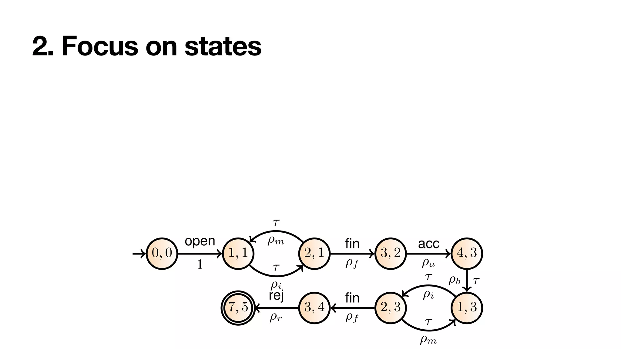
Reasoning on Labelled Petri Nets and their Dynamics in a Stochastic Setting 13
s1 s2
s3
s4
⌧ ⌧
⌧
⌧
en fin
acc
fin
ej
0, 0 1, 1 2, 1 3, 2 4, 3
1, 3
2, 3
3, 4
7, 5
open
1 ⌧
⇢i
⌧
⇢m fin
⇢f
acc
⇢a
⌧
⇢b
⌧
⇢i
⌧
⇢m
fin
⇢f
rej
⇢r](https://image.slidesharecdn.com/bpm2022-stochastic-reasoning-220922205316-6b26f0e0/75/Reasoning-on-Labelled-Petri-Nets-and-Their-Dynamics-in-a-Stochastic-Setting-61-2048.jpg)
![1. Infuse the cross-product with net probabilities
6 Sander J.J. Leemans et al.
s0
[q0]
s1
[q1]
s2
[q2]
s3
[q3]
s4
[q4]
s7
[q7]
s5
[q5]
s6
[q6]
s8
[q8]
1
open
⇢i = i
i+c
⌧
⇢m = m
m+f
⌧
⇢f = f
m+f
fin ⇢a
=
a
a+r
acc
⇢r = r
a+r
rej
⇢b = b
b+p+d
⌧
⇢c = c
i+c can
⇢d = d
b+p+d
⌧
⇢p = d
b+p+d
pay
1
del
Fig. 3: Stochastic reachability graph of the order-to-cash bounded stochastic PNP.
States are named. The initial state is shown with a small incoming edge. Final states
have a double countour.
Definition 7 (Labelled transition system). A labelled transition system is a tuple
hS, s0, Sf , %i where: (i) S is a (possibly infinite) set of states; (ii) s0 2 S is the ini-
tial state; (iii) Sf ✓ S is the set of accepting states; (iv) % ✓ S ⇥⌃ ⇥ S is a⌃-labelled
transition relation. A run is a finite sequence of transitions leading from s0 to one of the
Reasoning on Labelled Petri Nets and their Dynamics in a Stochastic Setting 13
s1 s2
s3
s4
⌧ ⌧
⌧
⌧
en fin
acc
fin
ej
0, 0 1, 1 2, 1 3, 2 4, 3
1, 3
2, 3
3, 4
7, 5
open
1 ⌧
⇢i
⌧
⇢m fin
⇢f
acc
⇢a
⌧
⇢b
⌧
⇢i
⌧
⇢m
fin
⇢f
rej
⇢r](https://image.slidesharecdn.com/bpm2022-stochastic-reasoning-220922205316-6b26f0e0/75/Reasoning-on-Labelled-Petri-Nets-and-Their-Dynamics-in-a-Stochastic-Setting-62-2048.jpg)
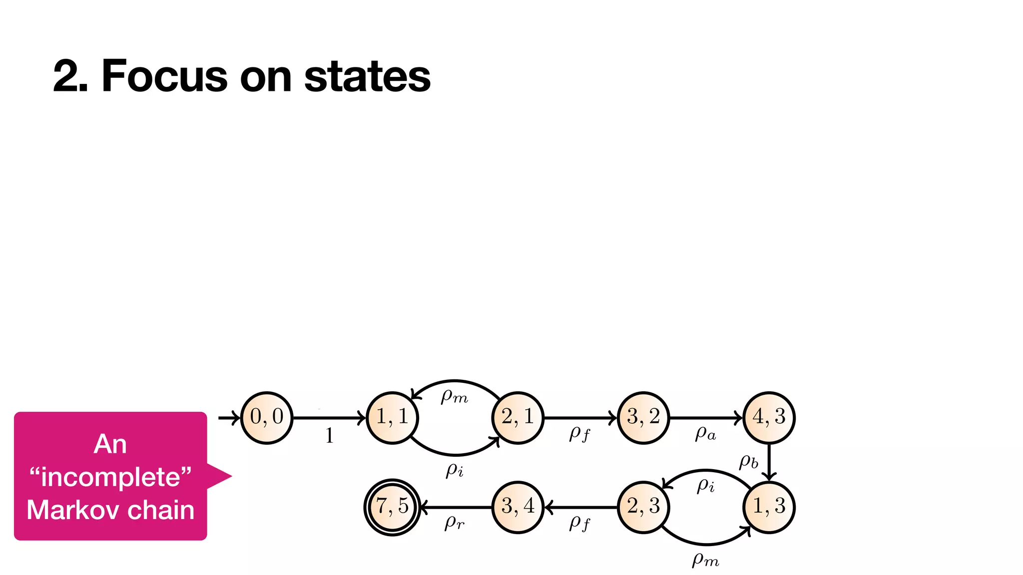
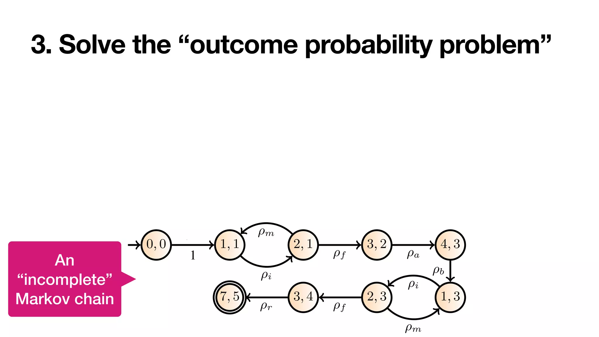
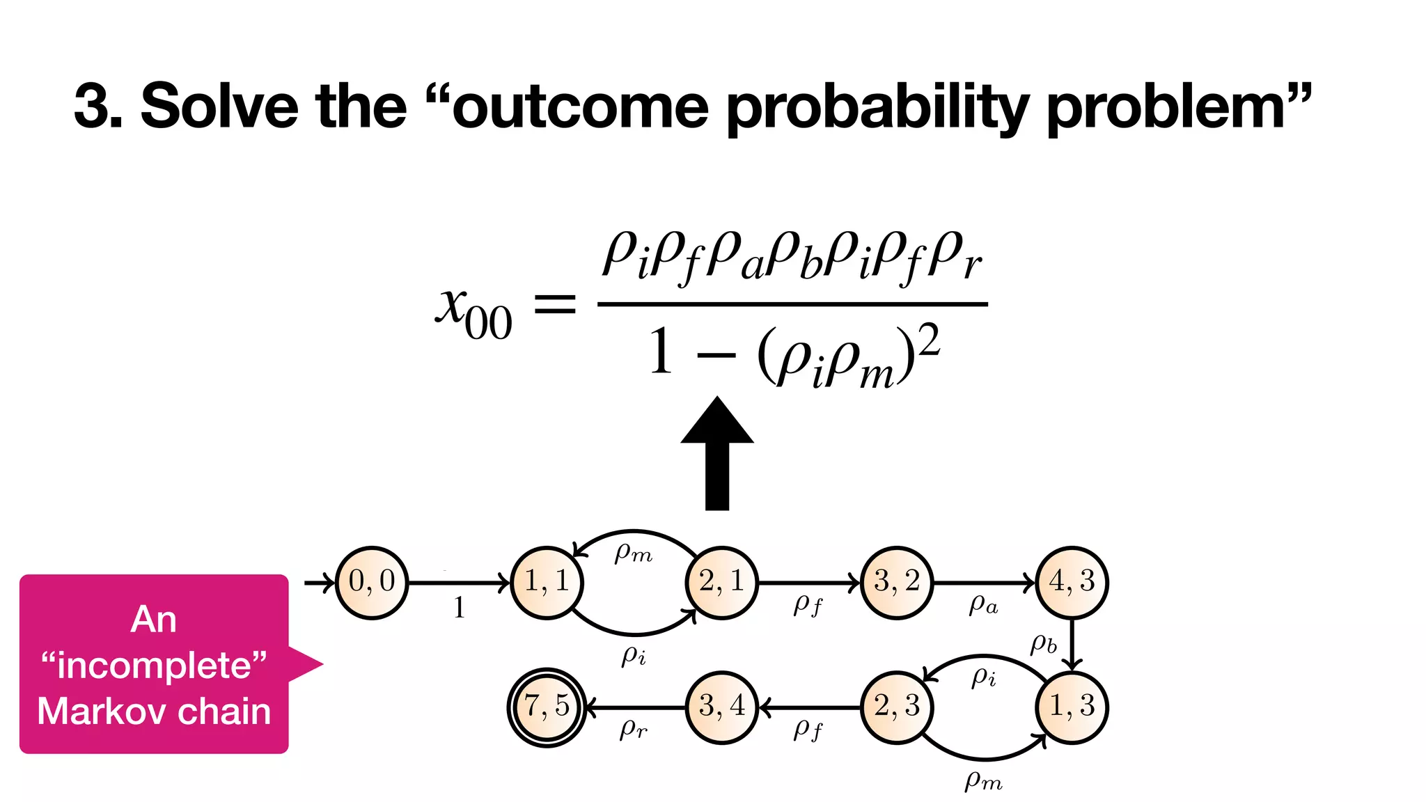
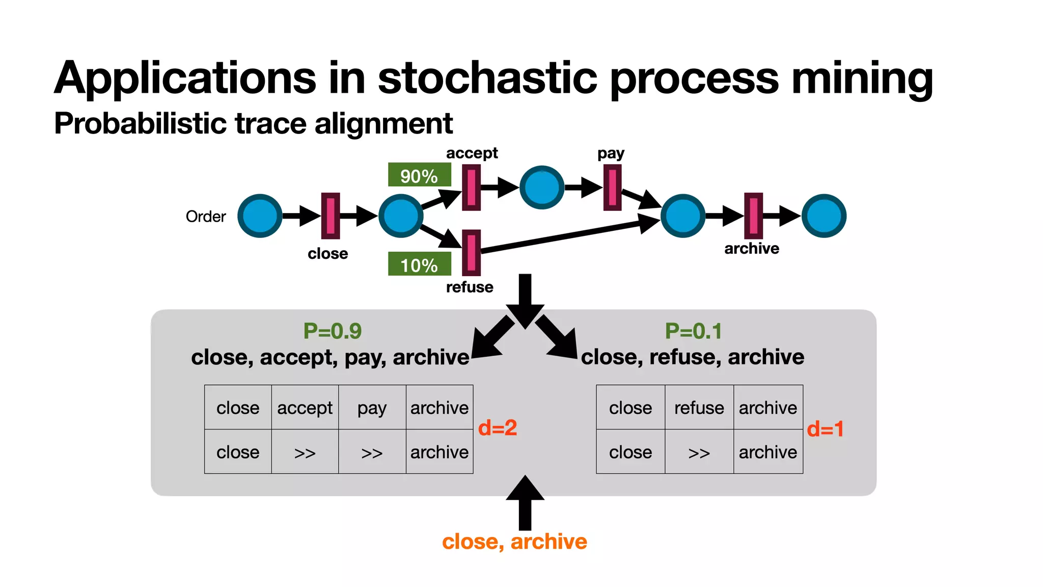

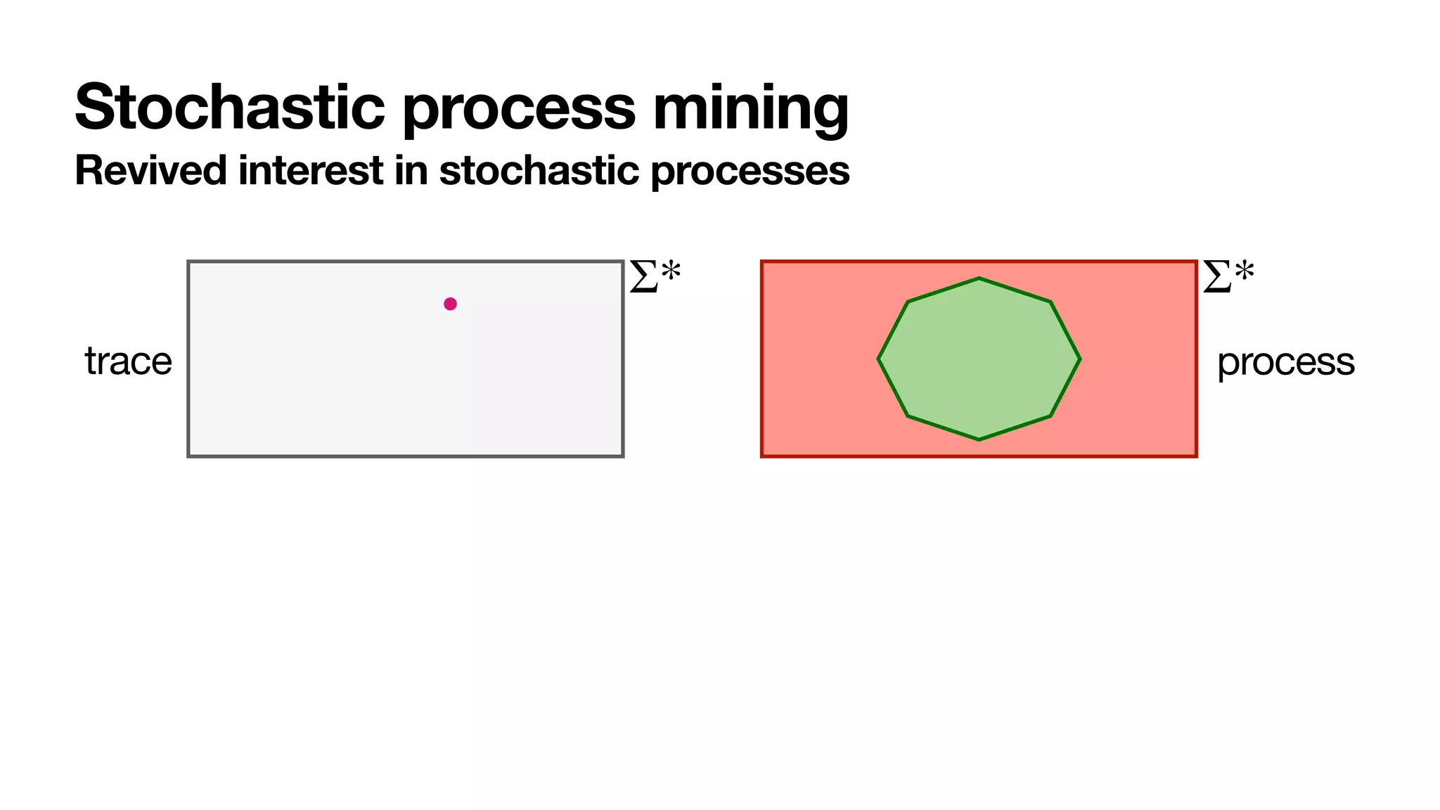
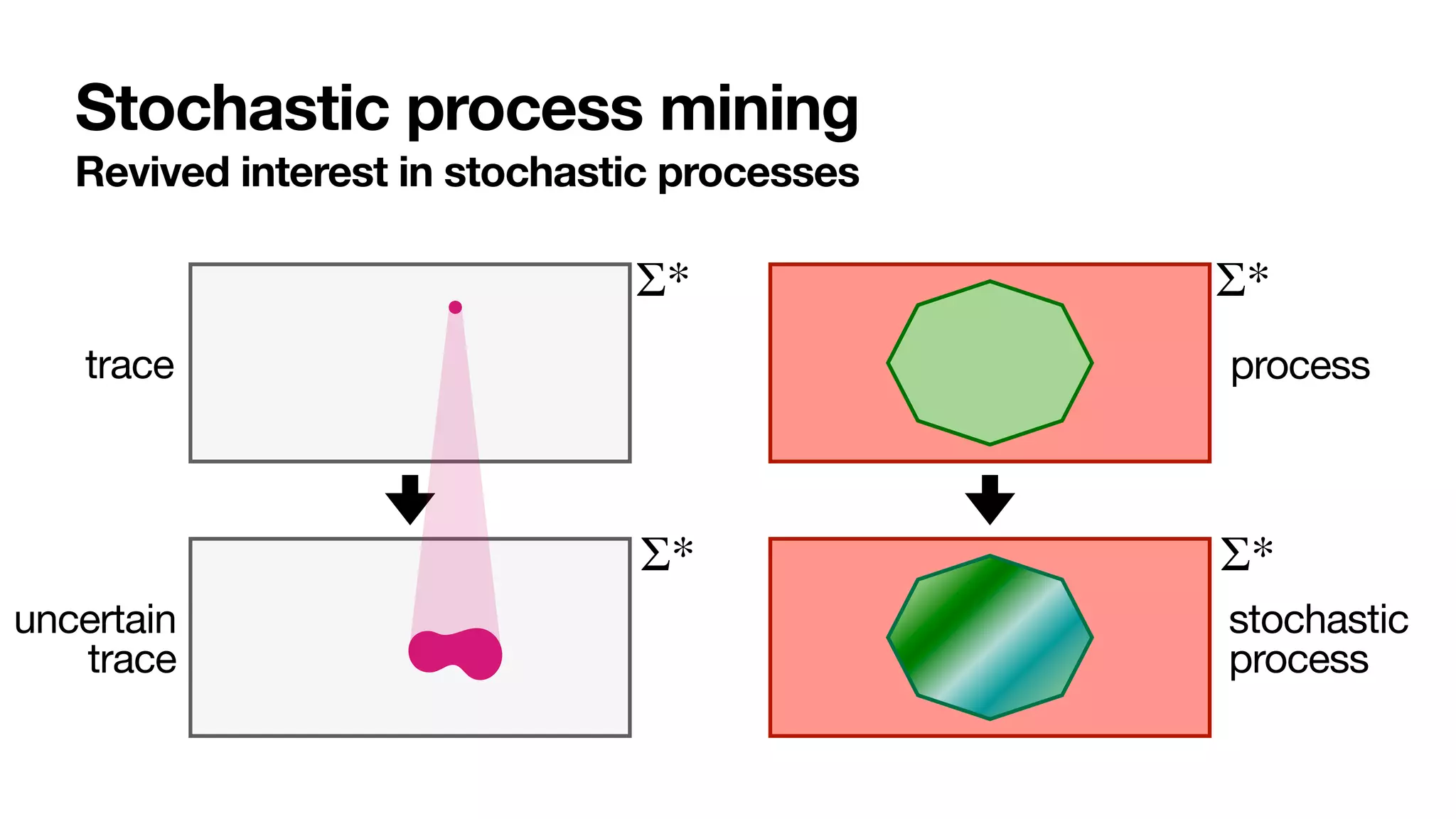
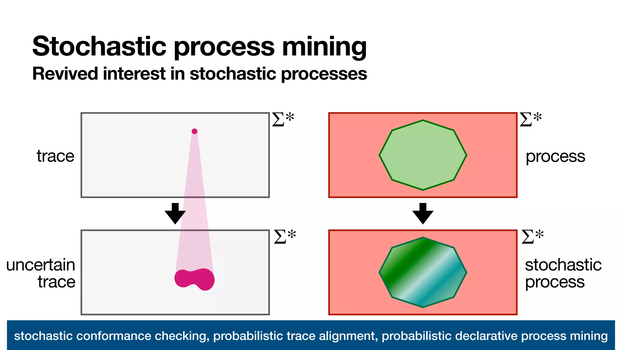
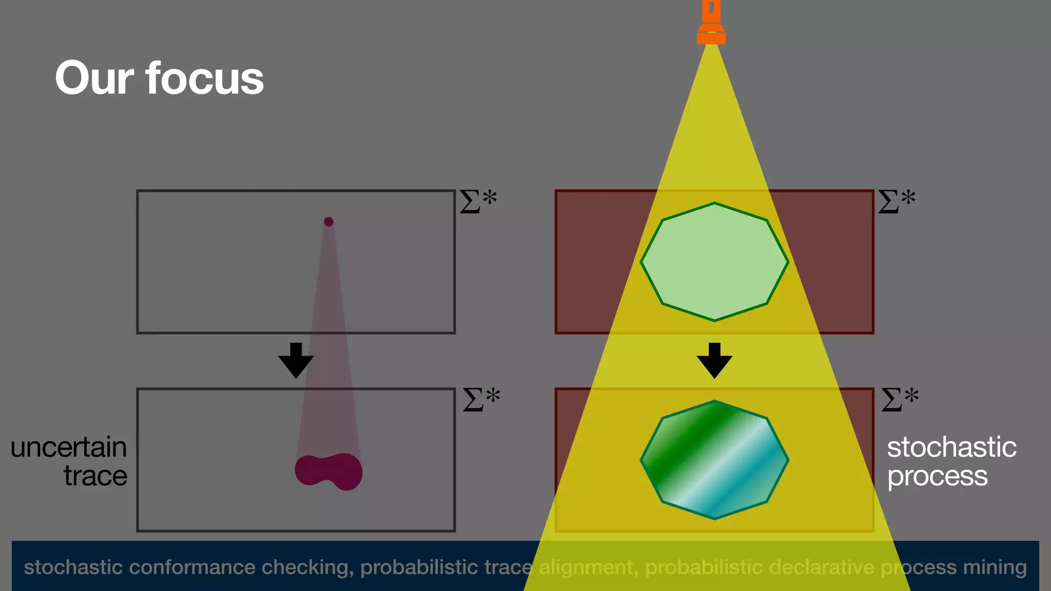
The document discusses labelled Petri nets and their application in process mining within a stochastic framework. It introduces concepts such as stochastic conformance checking, probabilistic trace alignment, and defines a labelled Petri net in detail, emphasizing its components and dynamics. The focus is on the structure of these nets and their role in modeling uncertain processes, particularly in an order-to-cash scenario.