Downloaded 119 times


![2-2. Incidence Matrix
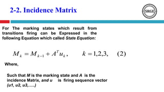
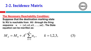
Incidence Matrix: for a Petri Net (𝑵. 𝑴𝟎) with
n Transitions and m Places , the Incidence
Matrix 𝑨 = [𝒂 𝒊𝒋] is (𝒏 𝒙 𝒎) matrix of integers
as:
)1(
ijijij aaa
),( jiij ptwa
),( ijij tpwa
Where,](https://image.slidesharecdn.com/petrinetanoverview2-180812112934/85/Petri-Nets-Properties-Analysis-and-Applications-22-320.jpg)
![3.3. Timing Petri Nets
(Enabling, Firing Rule)
P1
P2
P3
[1] {4}
𝟐
1
3
1
5
5
𝑴𝟎 = {(𝑷𝟏, 𝟏), (𝑷𝟏, 𝟑), (𝑷𝟐, 𝟏), (𝑷𝟑, 𝟎)}
𝑴𝟏 = {(𝑷𝟏, 𝟑), (𝑷𝟐, 𝟎), 𝟐(𝑷𝟑, 𝟓)}
1 3
2 4
5](https://image.slidesharecdn.com/petrinetanoverview2-180812112934/85/Petri-Nets-Properties-Analysis-and-Applications-38-320.jpg)
![3.3. Timing Petri Nets
(Enabling, Firing Rule)
Tasks
[0,5] {5}
0
Busy 1
Free 1
Free 2
Busy 2
Output
Start 1 Finish 1
Start 2 Finish 2
1
0
[1] {5}
[5] {0}
[6] {0}
5
0
6
55
6
6
Example:
0 2
1 3
4
5
6
TIME](https://image.slidesharecdn.com/petrinetanoverview2-180812112934/85/Petri-Nets-Properties-Analysis-and-Applications-39-320.jpg)
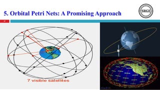
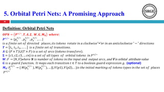
![5. Orbital Petri Nets: A Promising Approach
(Enabling, Firing Rule)
49
P1
P2
P3
t1
[1,50]
[2,100]
𝑴 𝟎 = (𝟏, 𝟏, 𝟎, || 𝟓𝟎, 𝟕𝟎)
[1,70]
𝑴 𝟏 = (𝟎, 𝟎, 𝟐, || 𝟏𝟎𝟎)](https://image.slidesharecdn.com/petrinetanoverview2-180812112934/85/Petri-Nets-Properties-Analysis-and-Applications-49-320.jpg)
![5. Orbital Petri Nets: A Promising Approach
(Enabling, Firing Rule)
50
t1
t2
[1,50]
[1,80]
[1,100]
[1,60]
[2,130]
[2,20]
𝑴𝟎 = (𝟏, 𝟏, 𝟏, 𝟏, 𝟎, 𝟎 || 𝟓𝟎, 𝟖𝟎, 𝟏𝟎𝟎, 𝟔𝟎)
𝑴𝟏 = (𝟎, 𝟏, 𝟎, 𝟏, 𝟐, 𝟎 || 𝟖𝟎, 𝟔𝟎, 𝟏𝟑𝟎)
𝑴𝟐 = (𝟎, 𝟎, 𝟎, 𝟎, 𝟐, 𝟐 || 𝟏𝟑𝟎, 𝟐𝟎)
Example:
P1
P2
P3
P4
P5
P6](https://image.slidesharecdn.com/petrinetanoverview2-180812112934/85/Petri-Nets-Properties-Analysis-and-Applications-50-320.jpg)


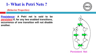
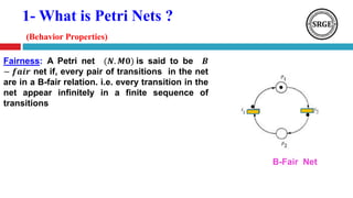
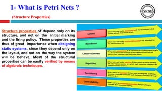
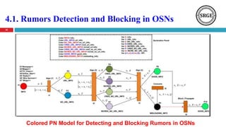
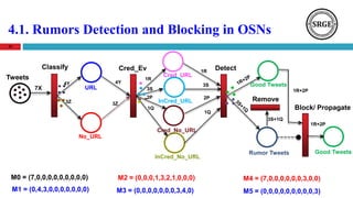
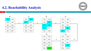
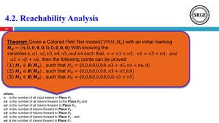
This document presents an agenda for a talk on Petri nets. It begins with an introduction to Petri nets that defines their structure, including places, transitions, tokens, and firing rules. It then discusses several analysis methods for Petri nets, including reachability trees, incidence matrices, and reduction rules. Next, it covers high-level Petri nets and colored Petri nets. The document concludes by mentioning an application of Petri nets to rumor detection and blocking in online social networks, and introduces orbital Petri nets as a promising approach.
![[slides] Software Engineering Third Edition - Aggarwal, Singh.pdf](https://cdn.slidesharecdn.com/ss_thumbnails/slidessoftwareengineeringthirdedition-aggarwalsingh-230615025923-02cadfc5-thumbnail.jpg?width=640&height=640&fit=bounds)