Download to read offline

![Real/Double
• A real number is any number along an infinitely number line
• They include fractions
• Denoted mathematically with ( mathbb{R} )
• Any numeric vector that does not have values followed by letter “L” are
considered as double e.g. c(-3, 0, 2, 5, 6). Can confirm a vector is a real
or double vector with funtion “is.double” e.g is.double(c(-3, 0, 2, 5,
6))
String/Character
• Composed of alphabetical letters and word/text
• Denoted by single or double quotation marks
• R has a special vector with alphabetical letter; this is letters
• Example c("a", "b", "c"), letters, c('cats', 'and' , 'dogs')
• Can check whether a vector is a character vector with function
is.character e.g. is.character(letters)
Data type: Factors
n
• In R a factor vector is a categorical variable with discrete classification
(grouping)
• Example
cat <- factor(c(rep("Y", 28), rep("N", 10)))
is.factor(cat)
[1] TRUE
levels(cat)
[1] "N" "Y"
Data type: Complex
n
• These are vectors with real and imaginary values. Imaginary numbers are
denoted by letter “i”
• Mathematically used to make it possible to take square-root of negative
values
3](https://image.slidesharecdn.com/r-training2-170404065558/85/R-training2-3-320.jpg)
![# Example, complex vector
3+2i
[1] 3+2i
# Confirm it's complex
is.complex(3+2i)
[1] TRUE
Data type: Raw
• These are vectors containing computer bytes or information on data storage
units
• More of computer language (0’s and 1’s) than human readable language
• Integers and doubles are jointly refered to as numeric
• The most commonly used data types are logical, numeric and characters.
Complex and raw data types are rarely used
int <- c(-3L, -2L, -1L, 0L, 1L, 2L, 3L)
is.integer(int)
[1] TRUE
is.numeric(int)
[1] TRUE
doub <- c(-3, -2, -1, 0, 1, 2, 3)
is.double(doub)
[1] TRUE
is.numeric(doub)
[1] TRUE
Data structures
• There two broad types of data structures in R
– Atomic vectors
– Generic (list) vectors
• These structures have three properties
– Type
– Length and
– Attributes
4](https://image.slidesharecdn.com/r-training2-170404065558/85/R-training2-4-320.jpg)
![• Function "type" is used to establish a vector’s type, function "length"
is used to determine length and function "attributes" is used to get
additional information about a vector
• Atomic vectors and lists differ in their type as atomic vectors can only
contain one data type while lists can contain any number of data types.
Atomic Vectors
• Contains only one data type, they include 1 dimensional atomic vectors, 2
dimensional atomic vectors called “matrices” and multi-dimensional atomic
vectors called “arrays”.
• Dimensionality can be considered as number of indices required to address
any element in a vector e.g. vector “cat” requires one index to address any
value, for example index “4” means fourth value which is Y
• Single variables are all atomic vectors of one dimension
• To check if a vector is either atomic or list, use is.atomic() or is.list().
Note there is a is.vector() but this checks if vector is named
Atomic vectors: Matrices
• Two dimensional atomic vectors, they contain data of the same type
• Any atomic vector can be converted to a matrix by adding a dim attribute
cat <- c(rep("Y", 28), rep("N", 10))
typeof(cat)
[1] "character"
dim(cat)
NULL
is.matrix(cat)
[1] FALSE
dim(cat) <- c(19, 2)
typeof(cat)
[1] "character"
dim(cat)
[1] 19 2
is.matrix(cat)
5](https://image.slidesharecdn.com/r-training2-170404065558/85/R-training2-5-320.jpg)
![[1] TRUE
• Other than using "dim()" to convert a one dim to a multi-dimension
atomic vector, matrices can be created with "matrix()", or by coercing
another data object with "as.matrix()"
typeof(airmiles)
[1] "double"
airmiles2 <- matrix(airmiles, nrow = 8, ncol = 3)
is.matrix(airmiles2)
[1] TRUE
airmiles3 <- as.matrix(airmiles, nrow = 8, ncol = 3)
is.matrix(airmiles3)
[1] TRUE
rm(airmiles2, airmiles3)
Special 1 & 2 dimension atomic vectors
Time series objects
• These are vectors used to store observations collected at given time points
(interval) over a period time, e.g. observations collected every three three
months for five year.
• Distiguishing feature in this data is time, interval is usually constant like
three months (regular), but in other cases it might not be so (irregular)
• In R, time series data are numeric vectors with attribute class equal “ts”
meaning time series
• Time series vectors can either be 1 dim atomic vector like “AirPassengers”
data set in R or a 2d matrix like "EuStockMarkets"
typeof(AirPassengers)
[1] "double"
attr(AirPassengers, "class")
[1] "ts"
typeof(EuStockMarkets)
[1] "double"
attr(EuStockMarkets, "class")
[1] "mts" "ts" "matrix"
6](https://image.slidesharecdn.com/r-training2-170404065558/85/R-training2-6-320.jpg)

![Importing and Exporting Data in R
• Data importation also referred to as “reading in” data
• Reading data depends on type and location of file
• Sub-session interest, reading in local R, text, excel, database and other
statistical program files
• Also discuss web scrapping
Reading in .RData
• Data created in R can be store in RData file
• This could be any data structure or a collection of data saved from an
active working directory (workspace)
• Function “save.image()” used to store workspace, function “load” is used
to read in any “.RData” (or even .Rhistory)
# See current objects
ls()
[1] "cat" "doub" "int"
# Store in an external .RData file
save.image()
# Remove all object from workspace/global environment
rm(list = ls())
ls()
character(0)
# Read in .RData
load(".RData")
# Check we have them back
ls()
[1] "cat" "doub" "int"
R’s core importing function “read.table()”
• read.table is R’s core importing function
• Almost all other functions including contributed packages depend on this
function
• Reads a file and creates a data frame from it
• It has a number of wrapper functions (functions which provide a con-
vinience interface to another function like give pre-defined/default values,
this make function calls more efficient)
8](https://image.slidesharecdn.com/r-training2-170404065558/85/R-training2-8-320.jpg)


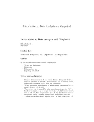
This document provides an introduction to data analysis and graphics in R. It covers vectors and assignment, data types including logical, integer, numeric, character, factor, complex and raw. It also discusses data structures such as atomic vectors, matrices, arrays and lists. Finally, it discusses importing data into R from files such as .RData files, text files using read.table(), CSV files and Excel files.