R is a software package for data analysis and graphical representation. It provides functions, results of analysis as objects, and a flexible environment for model building. This document provides tutorials on basic R operations including computation, vectors, matrices, and graphics. Key functions introduced are cbind(), rbind(), seq(), rep(), and matrix() for creating and manipulating objects, and plot() for data visualization.

1. R Tutorial for a Windows
Environment
Some tutorials are available on internet. Those I have
found particularly useful are
https://www.datacamp.com/courses/introduction-to-r
Offers an interactive tutorial to R for beginners
http://www.r-tutor.com/r-introduction/basic-data-types/numeric
R-tutorial based on the eBook R Tutorioal for Bayesian
Statistics, you are advised to browse.

2. What is R
0. R Basics
0.1. What is R?
R is a software package especially suitable for data analysis and graphical
representation. Functions and results of analysis are all stored as objects, allowing
easy function modification and model building. R provides the language, tool, and
environment in one convenient package.
It is very flexible and highly customizable. Excellent graphical tools make R an ideal
environment for EDA (Exploratory Data Analysis). Since most high level functions are
written in R language itself, you can learn the language by studying the function code.
On the other hand, R has a few weaknesses. For example, R is not particularly efficient in
handling large data sets. Also, it is rather slow in executing a large number of `for –
do’ loops, compared to compiler languages such as C/C++. Learning curve is
somewhat steep compared to "point and click" software.
RevolutionAnalytics_WhatisR.mp4

3. Where to get R
0.2 Where do I get R?
There are versions for Unix, Windows, and
Macintosh. All of them are free, and Windows
version is downloadable at:
http://cran.us.r-project.org/bin/windows
and follow the download instructions.

4. Typical R-window

5. Invoking R
0.3 Invoking R
If properly installed, usually R has a shortcut icon on the desktop screen and/or
you can find it under Start|Programs|R menu. If not, search and run the
executable file rgui.exe by double clicking from the search result window.
To quit R, type q() at the R prompt (>) and press Enter key. A dialog box will
ask whether to save the objects you have created during the session so that
they will become available next time you invoke R. Click Cancel this time.
Commands you entered can be easily recalled and modified. Just by hitting the
arrow keys in the keyboard, you can navigate through the recently entered
commands.
>objects() # list the names of all objects
> rm(data1) #removes the object named data1 from the current environment

6. Graphics
1. Graphics: a few examples
In addition to standard plots such as
histogram, bar charts, pie charts and so
forth, R provides an impressive array of
graphical tools. The following series of plots
shows a few of the extensive graphical
capabilities of R.

7. Time Series Plot

8. Boxplots

9. Iris Data

10. A Three dimensional Plot

11. Star Plot

12. Three dimensional Graph

13. Demos
Interactive graphics can serve as a great
learning tool. Students can quickly grasp the
role of outliers and influential points in a
simple linear regression by the following
example.
> library(tcltk)
> demo(tkcanvas)

14. Demo-Linear Regression

15. Effect of kernel choice, sample size and
bandwidth can be conveniently illustrated by
the following demonstration:
> library(tcltk)
> demo(tkdensity)

16. Change Window Width and
type of Kernel to see its effect

17. Basic Operations
• 2. Basic Operations
• 2.1 Computation
First of all, R can be used as an ordinary calculator.
There are a few examples:
> 2 + 3 * 5 # Note the order of operations.
> log (10) # Natural logarithm with base e=2.718282
> 4^2 # 4 raised to the second power
> 3/2 # Division
> sqrt (16) # Square root
> abs (3-7) # Absolute value of 3-7
> pi # The mysterious number
> exp(2) # exponential function
> 15 %/% 4 # This is the integer divide operation
> # This is a comment line

18. Assignment Operator
Assignment operator (<-) stores the value
(object) on the right side of (<-) expression
in the left side. Once assigned, the object
can be used just as an ordinary component
of the computation.

19. What Objects Look Like
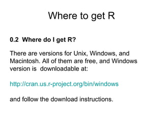
To find out what the object looks like, simply type its name. Note
that R is case sensitive, e.g., object names abc, ABC, Abc are all
different.
> x<- log(2.843432) *pi
> x
[1] 3.283001
> sqrt(x)
[1] 1.811905
> floor(x) # largest integer less than or equal to x (Gauss
number)
[1] 3
> ceiling(x) # smallest integer greater than or equal to x
[1] 4

20. Conflict with Built-in-Functions
Important note: since there are many built-in
functions in R, make sure that the new object
names you assign are not already used by the
system. A simple way of checking this is to type in
the name you want to use. If the system returns an
error message telling you that such object is not
found, it is safe to use the name. For example, c
(for concatenate) is a built-in function used to
combine elements so NEVER assign an object to
c!

21. Vectors
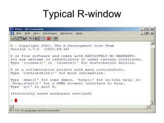
• 2.2 Vector
R handles vector objects quite easily and intuitively.
• > x<-c(1,3,2,10,5) #create a vector x with 5 components
> x
[1] 1 3 2 10 5
> y<-1:5 #create a vector of consecutive integers
> y
[1] 1 2 3 4 5
> y+2 #scalar addition
[1] 3 4 5 6 7
> 2*y #scalar multiplication
[1] 2 4 6 8 10
> y^2 #raise each component to the second power
[1] 1 4 9 16 25
> 2^y #raise 2 to the first through fifth power
[1] 2 4 8 16 32
> y #y itself has not been unchanged
[1] 1 2 3 4 5
> y<-y*2
> y #it is now changed
[1] 2 4 6 8 10

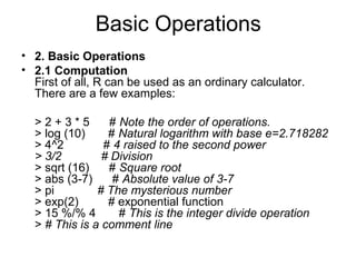
22. More Examples-1
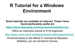
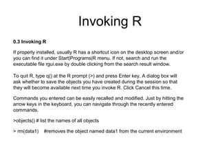
More examples of vector arithmetic:
> x<-c(1,3,2,10,5); y<-1:5 #two or more
statements are separated by semicolons
> x+y
[1] 2 5 5 14 10
> x*y
[1] 1 6 6 40 25
> x/y
[1] 1.0000000 1.5000000 0.6666667 2.5000000
1.0000000
> x^y
[1] 1 9 8 10000 3125

23. More Examples-2
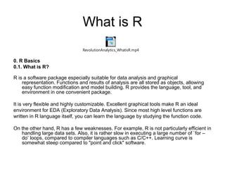
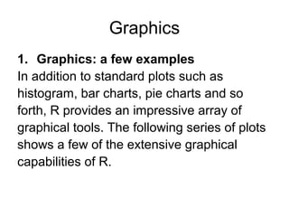
> sum(x) #sum of elements in x
[1] 21
> cumsum(x) #cumulative sum vector
[1] 1 4 6 16 21
> diff(x) # first difference
[1] 2 -1 8 -5
> diff(x,2) #second difference
[1] 1 7 3
> max(x) #maximum
[1] 10
> min(x) #minimum
[1] 1

24. Other Operations on Vectors
• Sorting can be done using sort() command:
> x
[1] 1 3 2 10 5
> sort(x) # increasing order
[1] 1 2 3 5 10
> sort(x, decreasing=T) # decreasing order
[1] 10 5 3 2 1
• Component extraction is a very important part of vector calculation.
> x
[1] 1 3 2 10 5
> length(x) # number of elements in x
[1] 5
> x[3] # the third element of x
[1] 2
> x[3:5] # the third to fifth element of x, inclusive
[1] 2 10 5
> x[-2] # all except the second element
[1] 1 2 10 5
> x[x>3] # list of elements in x greater than 3
[1] 10 5

25. Logical and Character Vector
• Logical vector can be handy:
> x>3
[1] FALSE FALSE FALSE TRUE TRUE
> as.numeric(x>3) # as.numeric() function coerces logical components to
numeric
[1] 0 0 0 1 1
> sum(x>3) # number of elements in x greater than 3
[1] 2
> (1:length(x))[x<=2] # indices of x whose components are less than or
equal to 2
[1] 1 3
> z<-as.logical(c(1,0,0,1)) # numeric to logical vector conversion
> z
[1] TRUE FALSE FALSE TRUE
• Character vector:
> colors<-c("green", "blue", "orange", "yellow", "red")
> colors
[1] "green" "blue" "orange" "yellow" "red"

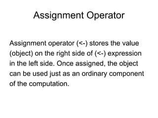
26. Names
Individual components can be named and referenced by their names.
> names(x) # check if any names are attached to x
NULL
> names(x)<-colors # assign the names using the character vector
colors
> names(x)
[1] "green" "blue" "orange" "yellow" "red"
> x
green blue orange yellow red
1 3 2 10 5
> x["green"] # component reference by its name
green
1
> names(x)<-NULL # names can be removed by assigning NULL
> x
[1] 1 3 2 10 5

27. Seq and Rep functions
seq() and rep() provide convenient ways to a construct vectors with a certain
pattern.
> seq(10)
[1] 1 2 3 4 5 6 7 8 9 10
> seq(0,1,length=10)
[1] 0.0000000 0.1111111 0.2222222 0.3333333 0.4444444 0.5555556
0.6666667
[8] 0.7777778 0.8888889 1.0000000
> seq(0,1,by=0.1)
[1] 0.0 0.1 0.2 0.3 0.4 0.5 0.6 0.7 0.8 0.9 1.0
> rep(1,3)
[1] 1 1 1
> c(rep(1,3),rep(2,2),rep(-1,4))
[1] 1 1 1 2 2 -1 -1 -1 -1
> rep("Small",3)
[1] "Small" "Small" "Small"
> c(rep("Small",3),rep("Medium",4))
[1] "Small" "Small" "Small" "Medium" "Medium" "Medium" "Medium"
> rep(c("Low","High"),3)
[1] "Low" "High" "Low" "High" "Low" "High"

28. Matrices
2.3 Matrices
A matrix refers to a numeric array of rows and columns. One of the easiest
ways to create a matrix is to combine vectors of equal length using cbind(),
meaning "column bind":
> x
[1] 1 3 2 10 5
> y
[1] 1 2 3 4 5
> m1<-cbind(x,y);m1
x y
[1,] 1 1
[2,] 3 2
[3,] 2 3
[4,] 10 4
[5,] 5 5
> t(m1) # transpose of m1
[,1] [,2] [,3] [,4] [,5]
x 1 3 2 10 5
y 1 2 3 4 5

29. Matrix Example
• > m1<-t(cbind(x,y)) # Or you can combine them and
assign in one step
> dim(m1) # 2 by 5 matrix
[1] 2 5
> m1<-rbind(x,y) # rbind() is for row bind and
equivalent to t(cbind()).
• Of course you can directly list the elements and specify
the matrix:
> m2<-matrix(c(1,3,2,5,-1,2,2,3,9),nrow=3);m2
[,1] [,2] [,3]
[1,] 1 5 2
[2,] 3 -1 3
[3,] 2 2 9

30. Extracting Matrix Elements
• Note that the elements are used to fill the first column, then the second column and so on. To fill
row-wise, we specify byrow=T option:
> m2<-matrix(c(1,3,2,5,-1,2,2,3,9),ncol=3,byrow=T);m2
[,1] [,2] [,3]
[1,] 1 3 2
[2,] 5 -1 2
[3,] 2 3 9
• Extracting the component of a matrix involves one or two indices.
> m2
[,1] [,2] [,3]
[1,] 1 3 2
[2,] 5 -1 2
[3,] 2 3 9
> m2[2,3] #element of m2 at the second row, third column
[1] 2
> m2[2,] #second row
[1] 5 -1 2
> m2[,3] #third column
[1] 2 2 9

31. Extracting Matrix Elements-More
• > m2[-1,] #submatrix of m2 without the first row
[,1] [,2] [,3]
[1,] 5 -1 2
[2,] 2 3 9
> m2[,-1] #ditto, sans the first column
[,1] [,2]
[1,] 3 2
[2,] -1 2
[3,] 3 9
> m2[-1,-1] #submatrix of m2 with the first row and
column removed
[,1] [,2]
[1,] -1 2
[2,] 3 9

32. Componentwise
Matrix computation is usually done component-wise.
> m1<-matrix(1:4, ncol=2); m2<-
matrix(c(10,20,30,40),ncol=2)
> 2*m1 # scalar multiplication
[,1] [,2]
[1,] 2 6
[2,] 4 8
> m1+m2 # matrix addition
[,1] [,2]
[1,] 11 33
[2,] 22 44
> m1*m2 # component-wise multiplication
[,1] [,2]
[1,] 10 90
[2,] 40 160

33. Some Matrix Operations
• Note that m1*m2 is NOT the usual matrix multiplication. To do the matrix multiplication, you
should use %*% operator instead.
• > m1 %*% m2
[,1] [,2]
[1,] 70 150
[2,] 100 220
• > solve(m1) #inverse matrix of m1
[,1] [,2]
[1,] -2 1.5
[2,] 1 -0.5
> solve(m1)%*%m1 #check if it is so
[,1] [,2]
[1,] 1 0
[2,] 0 1
> diag(3) #diag() is used to construct a k by k identity matrix
[,1] [,2] [,3]
[1,] 1 0 0
[2,] 0 1 0
[3,] 0 0 1
> diag(c(2,3,3)) #as well as other diagonal matrices
[,1] [,2] [,3]
[1,] 2 0 0
[2,] 0 3 0
[3,] 0 0 3

34. Eigen values and Eigen vectors
• Eigenvalues and eigenvectors of a matrix
is handled by eigen() function:
> eigen(m2)
$values
[1] 53.722813 -3.722813
• $vectors
[,1] [,2]
[1,] -0.5657675 -0.9093767
[2,] -0.8245648 0.4159736

35. An Example of User Defined
Function
2.4 Finding roots: a simple example
A built-in R function uniroot() can be
called from a user defined function
root.fun() to compute the root of a
univariate function and plot the graph of
the function at the same time.

36. R-codes
> y.fun<-function (x)
{y<-(log(x))^2-x*exp(-x^3)
} > root.fun<- function ()
{ x<-seq(0.2,2,0.01)
y<-y.fun(x)
win.graph()
plot(x,y,type="l")
abline(h=0)
r1 <- uniroot(y.fun,lower=0.2,upper=1)$root
r2 <- uniroot(y.fun,lower=1,upper=2)$root
cat("Roots : ", round(r1,4), " ", round(r2,4),"n")
}
> root.fun()

37. Graph of the Function y.fun

38. Data Frame() Function
2.5 Data frame
Data frame is an array consisting of
columns of various mode (numeric,
character, etc). Small to moderate size
data frame can be constructed by
data.frame() function. For example, we
illustrate how to construct a data frame
from the car data*:

39. Car Data
Make Model Cylinder Weight Mileage Type
Honda Civic V4 2170 33 Sporty
Chevrolet Beretta V4 2655 26 Compact
Ford Escort V4 2345 33 Small
Eagle Summit V4 2560 33 Small
Volkswagen Jetta V4 2330 26 Small
Buick Le Sabre V6 3325 23 Large
Mitsbusihi Galant V4 2745 25 Compact
Dodge Grand Caravan V6 3735 18 Van
Chrysler New Yorker V6 3450 22 Medium
Acura Legend V6 3265 20 Medium

40. Data Frame for Car data
• > Make<-
c("Honda","Chevrolet","Ford","Eagle","Volkswagen","Bui
ck","Mitsbusihi",
+ "Dodge","Chrysler","Acura")
> Model<-
c("Civic","Beretta","Escort","Summit","Jetta","Le
Sabre","Galant",
+ "Grand Caravan","New Yorker","Legend")
• Note that the plus sign (+) in the above commands are
automatically inserted when the carriage return is
pressed without completing the list. Save some typing by
using rep() command. For example, rep("V4",5) instructs
R to repeat V4 five times.

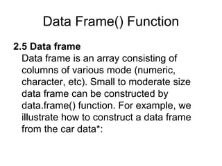
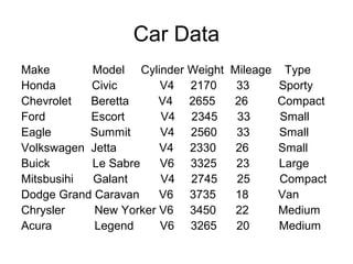
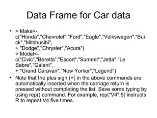
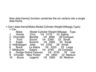
41. Making A Data Frame
• > Make<-
c("Honda","Chevrolet","Ford","Eagle","Volkswagen","Buick","Mitsbusihi",
+ "Dodge","Chrysler","Acura")
> Model<-c("Civic","Beretta","Escort","Summit","Jetta","Le Sabre","Galant",
+ "Grand Caravan","New Yorker","Legend")
• Note that the plus sign (+) in the above commands are automatically
inserted when the carriage return is pressed without completing the list.
Save some typing by using rep() command. For example, rep("V4",5)
instructs R to repeat V4 five times.
• > Cylinder<-c(rep("V4",5),"V6","V4",rep("V6",3))
> Cylinder
[1] "V4" "V4" "V4" "V4" "V4" "V6" "V4" "V6" "V6" "V6"
> Weight<-c(2170,2655,2345,2560,2330,3325,2745,3735,3450,3265)
> Mileage<-c(33,26,33,33,26,23,25,18,22,20)
> Type<-
c("Sporty","Compact",rep("Small",3),"Large","Compact","Van",rep("Medium",
2))

42. Now data.frame() function combines the six vectors into a single
data frame.
> Car<-data.frame(Make,Model,Cylinder,Weight,Mileage,Type)
> Car
Make Model Cylinder Weight Mileage Type
1 Honda Civic V4 2170 33 Sporty
2 Chevrolet Beretta V4 2655 26 Compact
3 Ford Escort V4 2345 33 Small
4 Eagle Summit V4 2560 33 Small
5 Volkswagen Jetta V4 2330 26 Small
6 Buick Le Sabre V6 3325 23 Large
7 Mitsbusihi Galant V4 2745 25 Compact
8 Dodge Grand Caravan V6 3735 18 Van
9 Chrysler New Yorker V6 3450 22 Medium
10 Acura Legend V6 3265 20 Medium

43. Column Labels
In addition, individual columns can be referenced
by their labels:
> Car$Mileage
[1] 33 26 33 33 26 23 25 18 22 20
> Car[,5] #equivalent expression, less
informative
> mean(Car$Mileage) #average mileage of the
10 vehicles
[1] 25.9
> min(Car$Weight)
[1] 2170

44. Table Function
• table() command gives a frequency table:
> table(Car$Type)
• Compact Large Medium Small Sporty Van
2 1 2 3 1 1
• If the proportion is desired, type the following command
instead:
> table(Car$Type)/10
• Compact Large Medium Small Sporty Van
0.2 0.1 0.2 0.3 0.1 0.1
• Note that the values were divided by 10 because there
are that many vehicles in total. If you don't want to count
them each time, the following does the trick:
> table(Car$Type)/length(Car$Type)

45. Cross Tabs
• Cross tabulation is very easy, too:
> table(Car$Make, Car$Type)
• Compact Large Medium Small Sporty Van
Acura 0 0 1 0 0 0
Buick 0 1 0 0 0 0
Chevrolet 1 0 0 0 0 0
Chrysler 0 0 1 0 0 0
Dodge 0 0 0 0 0 1
Eagle 0 0 0 1 0 0
Ford 0 0 0 1 0 0
Honda 0 0 0 0 1 0
Mitsbusihi 1 0 0 0 0 0
Volkswagen 0 0 0 1 0 0

46. Ordering Elements
What if you want to arrange the data set by vehicle weight? order() gets
the job done.
> i<-order(Car$Weight);i
[1] 1 5 3 4 2 7 10 6 9 8
> Car[i,]
Make Model Cylinder Weight Mileage Type
1 Honda Civic V4 2170 33 Sporty
5 Volkswagen Jetta V4 2330 26 Small
3 Ford Escort V4 2345 33 Small
4 Eagle Summit V4 2560 33 Small
2 Chevrolet Beretta V4 2655 26 Compact
7 Mitsbusihi Galant V4 2745 25 Compact
10 Acura Legend V6 3265 20 Medium
6 Buick Le Sabre V6 3325 23 Large
9 Chrysler New Yorker V6 3450 22 Medium
8 Dodge Grand Caravan V6 3735 18 Van

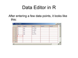
47. Creating/Editing Data
• 2.6 Creating/editing data objects
> y
[1] 1 2 3 4 5
• If you want to modify the data object, use edit() function
and assign it to an object. For example, the following
command opens notepad for editing. After editing is
done, choose File | Save and Exit from Notepad.
> y<-edit(y)
• If you prefer entering the data.frame in a spreadsheet
style data editor, the following command invokes the
built-in editor with an empty spreadsheet.
> data1<-edit(data.frame())

48. Data Editor in R
After entering a few data points, it looks like
this:

49. Variable Name
You can also change the variable name by clicking once on
the cell containing it. Doing so opens a dialog box:
When finished, click in the upper right corner of the dialog box to
return to the Data Editor window.
Close the Data Editor to return to the R command window (R
Console). Check the result by typing:
> data1

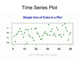
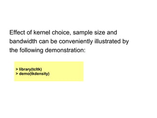
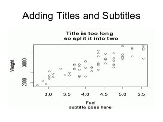
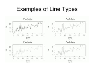
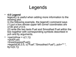
50. R Graphics
• 3. More on R GraphicsNot only R has fancy graphical tools, but also it has
all sorts of useful commands that allow users to control almost every aspect
of their graphical output to the finest details.
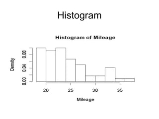
• 3.1 Histogram
We will use a data set fuel.frame which is based on makes of cars taken
from the April 1990 issue of Consumer Reports.
> library(SemiPar);data(fuel.frame);
• > names(fuel.frame)
[1] "car.name" "Weight" "Disp." "Mileage" "Fuel" "Type" >
attach(fuel.frame)
attach() allows to reference variables in fuel.frame without the
cumbersome
fuel.frame$ prefix.
• In general, graphic functions are very flexible and intuitive to use. For
example, hist() produces a histogram, boxplot() does a boxplot, etc.
> hist(Mileage)
> hist(Mileage, freq=F) # if probability instead of frequency is desired

51. Histogram

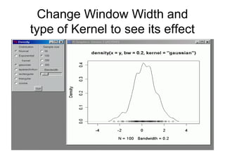
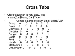
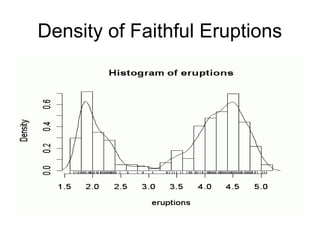
52. Density Plot
• Let us look at the Old Faithful geyser data, which
is a built-in R data set.
• > data(faithful)
> attach(faithful)
> names(faithful)
[1] "eruptions" "waiting"
> hist(eruptions, seq(1.6, 5.2, 0.2), prob=T)
> lines(density(eruptions, bw=0.1))
> rug(eruptions, side=1)

53. Density of Faithful Eruptions

54. Box Plot
3.2 Boxplot
> boxplot(Weight) # usual vertical boxplot
> boxplot(Weight, horizontal=T)
# horizontal boxplot
> rug(Weight, side=2) #data points

55. Box Plot

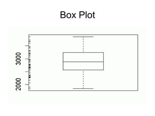
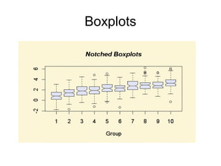
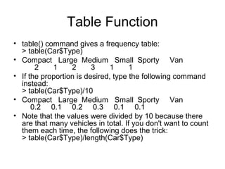
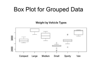
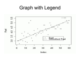
56. Grouped Data
• If you want to get the statistics involved in the boxplots, the following commands
show them. In this example, a$stats gives the value of the lower end of the whisker,
the first quartile (25th percentile), second quartile (median=50th percentile), third
quartile (75th percentile), and the upper end of the whisker.
> a<-boxplot(Weight, plot=F)
> a$stats
[,1]
[1,] 1845.0
[2,] 2567.5
[3,] 2885.0
[4,] 3242.5
[5,] 3855.0
> a #gives additional information
> fivenum(Weight) #directly obtain the five number summary
[1] 1845.0 2567.5 2885.0 3242.5 3855.0
• Boxplot is more useful when comparing grouped data. For example, side-by-side
boxplots of weights grouped by vehicle types are shown below:
> boxplot(Weight ~Type)
> title("Weight by Vehicle Types")

57. Box Plot for Grouped Data

58. Linear Regression
• On-line help is available for the commands:
> help(hist)
> help(boxplot)
• 3.3 plot()
plot() is a general graphic command with numerous
options.
> plot(Weight)
• The following command produce a scatterplot with
Weight on the x-axis and Mileage on the y-axis.
> plot(Weight, Mileage, main="Weight vs. Mileage")
• A fitted straight line is shown in the plot by executing two
more commands.
> fit<-lm(Mileage~Weight)
> abline(fit)

59. Regression Plot

60. Matrix Plot
3.4 matplot()
matplot() is used to plot two or more vectors of equal length.
> y60<-c(316.27, 316.81, 317.42, 318.87, 319.87, 319.43, 318.01,
315.74, 314.00, 313.68, 314.84, 316.03)
> y70<-c(324.89, 325.82, 326.77, 327.97, 327.91, 327.50, 326.18,
324.53, 322.93, 322.90, 323.85, 324.96)
> y80<-c(337.84, 338.19, 339.91, 340.60, 341.29, 341.00, 339.39,
337.43, 335.72, 335.84, 336.93, 338.04)
> y90<-c(353.50, 354.55, 355.23, 356.04, 357.00, 356.07, 354.67,
352.76, 350.82, 351.04, 352.69, 354.07)
> y97<-c(363.23, 364.06, 364.61, 366.40, 366.84, 365.68, 364.52,
362.57, 360.24, 360.83, 362.49, 364.34)
> CO2<-data.frame(y60, y70, y80, y90, y97)
> row.names(CO2)<-c("Jan", "Feb",
"Mar","Apr","May","Jun","Jul","Aug","Sep","Oct","Nov","Dec")

61. CO2 Data
> CO2
y60 y70 y80 y90 y97
Jan 316.27 324.89 337.84 353.50 363.23
Feb 316.81 325.82 338.19 354.55 364.06
Mar 317.42 326.77 339.91 355.23 364.61
Apr 318.87 327.97 340.60 356.04 366.40
May 319.87 327.91 341.29 357.00 366.84
Jun 319.43 327.50 341.00 356.07 365.68
Jul 318.01 326.18 339.39 354.67 364.52
Aug 315.74 324.53 337.43 352.76 362.57
Sep 314.00 322.93 335.72 350.82 360.24
Oct 313.68 322.90 335.84 351.04 360.83
Nov 314.84 323.85 336.93 352.69 362.49
Dec 316.03 324.96 338.04 354.07 364.34

62. Matrix Plot of CO2 Data
> matplot(CO2)
Note that the observations labeled 1 represents the monthly CO2 levels for
1960, 2 represents those for 1970, and so on. We can enhance the plot by
changing the line types and adding axis labels and titles:
> matplot(CO2,axes=F,frame=T,type='b',ylab="")
> #axes=F: initially do not draw axis
> #frame=T: box around the plot is drawn;
> #type=b: both line and character represent a seris;
> #ylab="": No label for y-axis is shown;
> #ylim=c(310,400): Specify the y-axis range
> axis(2) # put numerical annotations at the tickmarks in y-axis;
> axis(1, 1:12, row.names(CO2))
> # use the Monthly names for the tickmarks in x-axis; length is 12;
> title(xlab="Month") #label for x-axis;
> title(ylab="CO2 (ppm)")#label for y-axis;
> title("Monthly CO2 Concentration n for 1960, 1970, 1980, 1990 and
1997")
> # two-line title for the matplot

63. CO2 Monthly Plot by Year

64. Plot Options
• 4. Plot Options4.1 Multiple plots in a single graphic window
You can have more than one plot in a graphic window. For example,
par(mfrow=c(1,2))allows you to have two plots side by side.
par(mfrow=c(2,3)) allows 6 plots to appear on a page (2 rows of 3
plots each). Note that the arrangement remains in effect until you
change it. If you want to go back to the one plot per page setting,
type par(mfrow=c(1,1)).
• 4.2 Adjusting graphical parameters
4.2.1 Labels and title; axis limits
Any plot benefits from clear and concise labels which greatly
enhances the readability.
> plot(Fuel, Weight)
• If the main title is too long, you can split it into two and adding a
subtitle below the horizontal axis label is easy:
> title(main="Title is too long n so split it into two",sub="subtitle
goes here")

65. Adding Titles and Subtitles

66. Types of Plots and Lines
• By default, when you issue a plot command R inserts variable name(s) if it is
available and figures out the range of x axis and y axis by itself. Sometimes
you may want to change these:
> plot(Fuel, Weight, ylab="Weight in pounds", ylim=c(1000,6000))
• Similarly, you can specify xlab and xlim to change x-axis. If you do not want
the default labels to appear, specify xlab=" ", ylab=" ". This give you a plot
with no axis labels. Of course you can add the labels after using appropriate
statements within title() statement.
• > plot(Mileage, Weight, xlab="Miles per gallon", ylab="Weight in pounds",
xlim=c(20,30),ylim=c(2000,4000))
> title(main="Weight versus Mileage n data=fuel.frame;", sub="Figure 4.1")
• 4.2.2 Types for plots and lines
In a series plot (especially time series plot), type provides useful options:
> par(mfrow=c(2,2))
> plot(Fuel, type="l"); title("lines")
> plot(Fuel, type="b"); title("both")
> plot(Fuel, type="o"); title("overstruck")
> plot(Fuel, type="h"); title("high density")

67. Examples of Graphs

68. Line Types
Also you can specify the line types using lty argument
within plot() command:
> plot(Fuel, type="l", lty=1) #the usual series plot
> plot(Fuel, type="l", lty=2) #shows dotted line instead.
lty can go up to 8.
> plot(Fuel, type="l", lty=1); title(main="Fuel data",
sub="lty=1")
> plot(Fuel, type="l", lty=2); title(main="Fuel data",
sub="lty=2")
> plot(Fuel, type="l", lty=3); title(main="Fuel data",
sub="lty=3")
> plot(Fuel, type="l", lty=4); title(main="Fuel data",
sub="lty=4")

69. Examples of Line Types

70. Colors and Characters
– Note that we can control the thickness of the lines by lwd=1
(default) through lwd=5 (thickest).
– 4.3 Colors and characters
– You can change the color by specifying
> plot(Fuel, col=2)
which shows a plot with different color. The default is col=1. The
actual color assignment depends on the system you are using.
You may want to experiment with different numbers. Of course
you can specify the col option together with other options such
as type or lty. pch option allows you to choose alternative
plotting characters when making a points-type plot. For example,
the command
> plot(Fuel, pch="*") # plots with * characters
> plot(Fuel, pch="M") # plots with M.

71. Axis Line
• 4.4 Controlling axis line
• bty ="n"; No box is drawn around the plot, although the x and y axes
are still drawn.
bty="o"; The default box type; draws a four-sided box around the
plot.
bty="c"; Draws a three-sided box around the plot in the shape of an
uppercase "C."
bty="l"; Draws a two-sided box around the plot in the shape of an
uppercase "L."
bty="7"; Draws a two-sided box around the plot in the shape of a
square numeral "7."
> par(mfrow = c(2,2))
> plot(Fuel)
> plot(Fuel, bty="l")
> plot(Fuel, bty="7")
> plot(Fuel, bty="c")

72. Tick Marks
• 4.5 Controlling tick marks
tck parameter is used to control the length of tick marks. tck=1
draws grid lines. Any positive value between 0 and 1 draws inward
tick marks for each axis. Also with some more work you can have
tick marks of different lengths, as the following example shows.
• > plot(Fuel, main="Default")
> plot(Fuel, tck=0.05, main="tck=0.05")
> plot(Fuel, tck=1, main="tck=1")
> plot(Fuel, axes=F, main="Different tick marks for each axis")
> #axes=F suppresses the drawing of axis
> axis(1)# draws x-axis.
> axis(2, tck=1, lty=2) # draws y-axis with horizontal grid of dotted
line
> box()# draws box around the remaining sides.

73. Legends
• 4.6 Legend
legend() is useful when adding more information to the
existing plot.
In the following example, the legend() command says
(1) put a box whose upper left corner coordinates are
x=30 and y=3.5;
(2) write the two texts Fuel and Smoothed Fuel within the
box together with corresponding symbols described in
pch and lty arguments.
• >par(mfrow = c(1,1))
>plot(Fuel)
>lines(lowess(Fuel))
>legend(30,3.5, c("Fuel","Smoothed Fuel"), pch="* ",
lty=c(0,1))

74. Graph with Legend