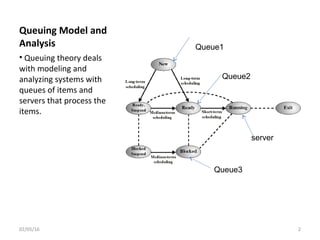
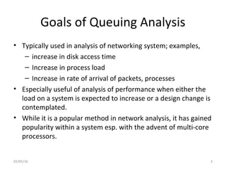
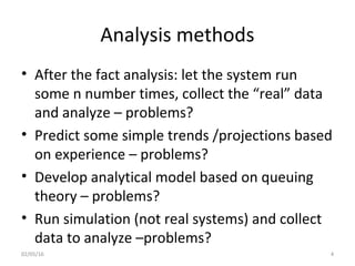
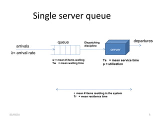
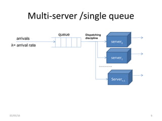
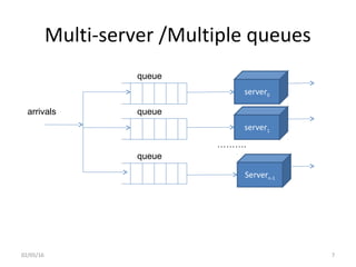
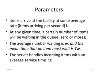
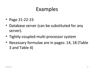
This document discusses queuing analysis and its applications. Queuing theory models systems with queues and servers that process items. It is useful for analyzing network and system performance when load or design changes are expected. The document outlines different analysis methods and key metrics like arrival rate, service time, waiting time, number of items, and utilization. It also covers important assumptions like Poisson arrivals, service time distributions, Little's Law, and example applications like database servers and multi-processor systems.

1. Queuing Analysis
Based on noted from Appendix A of
Stallings Operating System text
02/05/16 1

2. Queuing Model and
Analysis
• Queuing theory deals
with modeling and
analyzing systems with
queues of items and
servers that process the
items.
02/05/16 2
Queue1
Queue2
Queue3
server

3. Goals of Queuing Analysis
• Typically used in analysis of networking system; examples,
– increase in disk access time
– Increase in process load
– Increase in rate of arrival of packets, processes
• Especially useful of analysis of performance when either the
load on a system is expected to increase or a design change is
contemplated.
• While it is a popular method in network analysis, it has gained
popularity within a system esp. with the advent of multi-core
processors.
02/05/16 3

4. Analysis methods
• After the fact analysis: let the system run
some n number times, collect the “real” data
and analyze – problems?
• Predict some simple trends /projections based
on experience – problems?
• Develop analytical model based on queuing
theory – problems?
• Run simulation (not real systems) and collect
data to analyze –problems?
02/05/16 4

5. 02/05/16 5
Single server queue
w = mean # items waiting
Tw = mean waiting time
queue
arrivals
λ= arrival rate
server
Dispatching
discipline
departures
Ts = mean service time
ρ = utilization
r mean # items residing in the system
Tr = mean residence time

6. Multi-server /single queue
02/05/16 6
queue
arrivals
λ= arrival rate
Dispatching
discipline
server0
server1
Servern-1
……….

7. Multi-server /Multiple queues
02/05/16 7
server0
server1
Servern-1
……….
queue
arrivals queue
queue

8. Parameters
• Items arrive at the facility at some average
rate (items arriving per second) l.
• At any given time, a certain number of items
will be waiting in the queue (zero or more);
• The average number waiting is w, and the
mean time that an item must wait is Tw.
• The server handles incoming items with an
average service time Ts;
02/05/16 8

9. More parameters
• Utilization, ρ, is the fraction of time that the
server is busy, measured over some interval of
time.
• Finally, two parameters apply to the system as a
whole.
• The average number of items resident in the
system, including the item being served (if any)
and the items waiting (if any), is r;
• and the average time that an item spends in the
system, waiting and being served, is Tr; we refer
to this as the mean residence time
02/05/16 9

10. Analysis
• As the arrival rate, which is the rate of traffic passing through the
system, increases, the utilization increases and with it, congestion.
The queue becomes longer, increasing waiting time. At ρ = 1, the
server becomes saturated, working 100% of the time.
• Thus, the theoretical maximum input rate that can be handled by
the system is:
λmax = 1/Ts
• However, queues become very large near system saturation,
growing without bound when ρ = 1. Practical considerations, such
as response time requirements or buffer sizes, usually limit the
input rate for a single server to 70-90% of the theoretical
maximum.
• For multi server queue for N servers:
λmax = N/Ts
02/05/16 10

11. Specific Metrics
• The fundamental task of a queuing analysis is as follows: Given the
following information as input:
· Arrival rate
· Service time
• Provide as output information concerning:
· Items waiting
· Waiting time
· Items in residence
· Residence time.
• We would like to know their average values (w, Tw, r, Tr) and the
respective variability the σ’s
• We are also interested in some probabilities: what is probability
that items waiting in line < M is 0.99?
02/05/16 11

12. Important Assumptions
• The arrival rate obeys the Poisson distribution, which is equivalent
to saying that the inter-arrival times are exponential;
• On other words, the arrivals occur randomly and independent of
one another.
• A convenient notation has been developed for summarizing the
principal assumptions that are made in developing a queuing
model.
• The notation is X/Y/N, where X refers to the distribution of the
inter-arrival times, Y refers to the distribution of service times, and
N refers to the number of servers.
• M/M/1 refers to a single-server queuing model with Poisson
arrivals and exponential service times.
• M/G/1 and M/M/1 and M/D/1
02/05/16 12

13. Little’s Law
• Very simple law that works from a Case
Western Reserve University professor Dr.
Little
• Average number of customers in a system =
average arrival rate * average time spent in
the system
• r = Tr * λ
• w = Tw * λ
• Tr = Tw + Ts
02/05/16 13

14. Examples
• Page 21-22-23
• Database server (can be substituted for any
server).
• Tightly-coupled multi-processor system
• Necessary formulae are in pages: 14, 18 (Table
3 and Table 4)
02/05/16 14