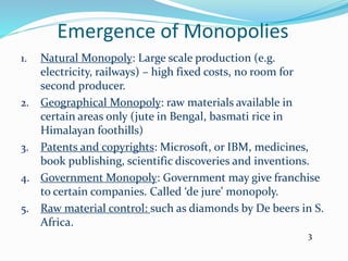
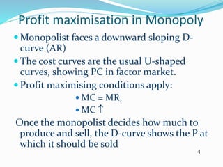
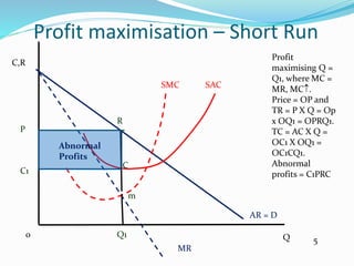
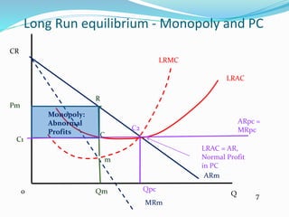
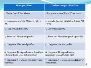
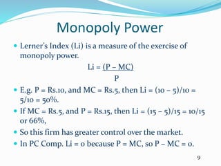
This document discusses the concept of monopoly and profit maximization by monopolistic firms. It covers the key features of monopoly markets including barriers to entry, downward sloping demand curves, and the ability of monopolies to be price makers. The document also examines how monopolies can engage in price discrimination by charging different prices to different consumer groups in order to maximize profits. Government policies aimed at regulating monopolies through anti-trust laws and taxes are also summarized.

1. Prof. Prabha Panth,
Osmania University,
Hyderabad
23-Apr-16

2. Pure Monopoly
 Monopoly – a market with a single firm.
 Produces and sells a commodity that has no close
substitutes,
 The firm = industry, no competition.
 Barriers to entry.
 The firm is a “Price Maker” – it is free to fix its own
price.
 AR curve or Demand curve is downward sloping,
the firm can sell more, but only at a lower price.
 MR lies below AR.
2

3. Emergence of Monopolies
1. Natural Monopoly: Large scale production (e.g.
electricity, railways) – high fixed costs, no room for
second producer.
2. Geographical Monopoly: raw materials available in
certain areas only (jute in Bengal, basmati rice in
Himalayan foothills)
3. Patents and copyrights: Microsoft, or IBM, medicines,
book publishing, scientific discoveries and inventions.
4. Government Monopoly: Government may give franchise
to certain companies. Called ‘de jure’ monopoly.
5. Raw material control: such as diamonds by De beers in S.
Africa.
3

4. Profit maximisation in Monopoly
 Monopolist faces a downward sloping D-
curve (AR)
 The cost curves are the usual U-shaped
curves, showing PC in factor market.
 Profit maximising conditions apply:
 MC = MR,
 MC 
Once the monopolist decides how much to
produce and sell, the D-curve shows the P at
which it should be sold
4

5. Profit maximisation – Short Run
C,R
0 Q
AR = D
MR
SACSMC
m
Q1
P
R
C
C1
Abnormal
Profits
Profit
maximising Q =
Q1, where MC =
MR, MC.
Price = OP and
TR = P X Q = Op
x OQ1 = OPRQ1.
TC = AC X Q =
OC1 X OQ1 =
OC1CQ1.
Abnormal
profits = C1PRC
5

6. Long Run Equilibrium
 In the long run, the monopolist experiences Returns to
Scale, and increases production.
 But he can still control his price.
 Hence he can still make abnormal profits.
 These profits attract new competitors,
 But the monopolist can create barriers to entry, and
prevent new competition.
 Pre empting licences,
 Buying copy rights and patents,
 Mergers with smaller firms.
 Economics of scale
6

7. Long Run equilibrium - Monopoly and PC
CR
0 Q
ARm
MRm
LRAC
LRMC
m
Qm
C
R
Pm
C1
Monopoly:
Abnormal
Profits
C2
ARpc =
MRpc
LRAC = AR,
Normal Profit
in PC
Qpc
7

8. Monopoly Firm Perfect competition Firm
1. Single firm, Price Maker 1. Large number of firms, Price taker
2. Downward sloping AR curve, MR <
AR
2. Straight line AR parallel to X axis, AR
= MR
3. Higher P, and lower Q 3. Lower P, higher Q
4. Short run Abnormal profits 4. Short run Abnormal profits possible
5. Long run: Abnormal profits 5. Long run: Normal profits
6. Long run: Firm produces at less than
efficient level, LAC not minimum
6. Long run: Firm produces at
minimum LAC, efficient firm
7. Long run: P > MC, so consumers are
exploited
7. Long run: P = MC, no exploitation of
consumers.
8

9. Monopoly Power
 Lerner’s Index (Li) is a measure of the exercise of
monopoly power.
Li = (P – MC)
P
 E.g. P = Rs.10, and MC = Rs.5, then Li = (10 – 5)/10 =
5/10 = 50%.
 If MC = Rs.5, and P = Rs.15, then Li = (15 – 5)/15 = 10/15
or 66%,
 So this firm has greater control over the market.
 In PC Comp. Li = 0 because P = MC, so P – MC = 0.
9

10. Price Discrimination
10

11. Price Discrimination
 Price discrimination: practice of monopolists of
charging different prices to different consumers for
the same or similar commodities, without
significant differences in the costs.
 Monopolist wants to take away or reduce
consumer’s surplus.
 This is possible when there are different buyers
who cannot communicate with each other,
 Or when it is not possible for buyers to trade with
each other.
11

12. Price Discrimination
 Based on:
a) Geographical distances: prices of text books in
USA > prices in India or Europe,
b) Income differences: Medical services, higher for
rich, and lower for poorer citizens.
c) Different age groups: less for senior citizens,
children, more for others (e.g. railways)
d) Quality: e.g. hard bound books more expensive
than paper back.
e) Time: Peak time airline tickets > off time tickets, or
early bird tickets.
12

13. First degree Price Discrimination
 The monopolist takes
away the entire
consumer surplus.
 Charges the highest
possible price, P1.
 Highly luxurious
goods e.g. Rolls
Royce, or collector’s
items such as rare
paintings, etc.
 “Take it or leave it”
policy
P
0
Q
D
Q1
P1
No consumer’s
surplus.
13

14. Second degree Price Discrimination
 Here the firm charges different rates for different
users of the same commodity by dividing
consumers into different categories:
 Timings (e.g. railway/airline tickets cheaper for
night travel, or during non-peak timings).
 Age: lower charges for senior citizens or for
children below 14 years.
 Perceived quality: hard bound books costlier
than paper back.
14

15. Second degree Price Discrimination
 Time: premier rates higher for new films, or
concerts, lower rates as time passes.
 Position: lower rates for front seats in a
theatre, or ‘economy class’ , ‘2nd class in
trains’. As compared to first class or AC.
People in different categories cannot buy at lower
rates and sell to others at higher rates.
Some, but not all, of consumer’s surplus is taken
away by the monopolist.
15

16. Second degree Price Discrimination
 Each unit (e.g. ticket) sold
at a different price.
 TR of 3 units = 500 + 400 +
300 = 1200
 If MC = MR gives P = 300.
Uniform price
 Then TR = 300 × 3 = 900
With price discrimination,
the firm earns 300 Rs more,
without any extra cost. 0
Q
D =MR
Q1
P1 = 500
Q2
P2 = 400
P3 = 300
Q3
MC
The blue triangles show that the monopolist cannot take
away the entire consumer’s surplus
16

17. Third Degree Price Discrimination
 When there are two or more different markets.
 Separated from each other in terms of space,
time, or income levels. (e.g. in posh areas, and in
low income areas, premier tickets)
 The elasticity of demand is different in each
market.
 The high income market has less elastic demand,
 The low income market has more elastic demand.
17

18. Third Degree Price Discrimination
0
P
ARa
MARKET A MARKET B
0
P
ARb
MONOPOLIST
FIRM
P
0 MR
a+b
AC =
MC
MRbMRa
QB
PB
QA
PB
T
QA+QB
18

19. Third degree Price Discrimination
 There are two unconnected markets A and B
 Market A has inelastic D curve, Market B has elastic D
curve.
 The monopolist produces the commodity with constant
costs (MC = AC).
 At the firm level, profit maximising Q is determined at T =
QA+QB.
 He sells QB in Market B at price PB, and QA in Market A at
price PA.
 QA < QB, while PA > PB.
 Market with more elastic D, has lower P, market with
inelastic demand has higher P.
 Thus the monopolist can make more profits by selling in
two different markets at two different prices.
19

20. Control of Monopoly
 Monopoly is discouraged by Governments, as it
leads to exploitation of consumers.
 Anti Monopoly Laws, Laws to encourage
Competition (MRTP Act, and Competition Act 2002
in India), Anti Restrictive Practices Acts, passed in
many countries.
 Or the Government can tax away the extra profits of
monopolists – through both direct profit taxes, or
through indirect taxes, and use the tax revenue for
other welfare purposes.
20

21. Questions
1. Short Answer Questions:
1. What are the main features of Monopoly?
2. What are the factors that lead to the emergence of
Monopoly?
3. What is meant by “barriers to entry”? What type of
barriers can be put up by a monopoly firm?
4. What is “Monopoly Power” and how is it measured?
5. What are the methods used by Governments to
regulate monopoly?
21

22. 2. Essay Questions:
1. Depict the short and the long run
equilibrium of a Monopoly Firm. How does it
differ from a firm in P.C?
2. What is Price Discrimination? Explain the
different types of price discrimination that
can be carried out by a monopolist.
3. Why is monopoly considered to be less
efficient than perfect competition? Give
reasons for your answer.
22