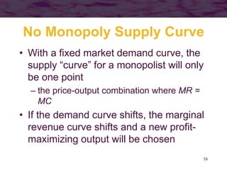
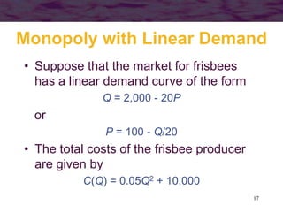
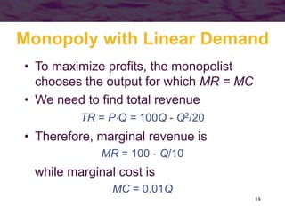
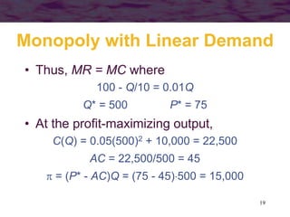
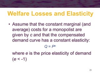
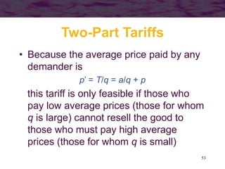
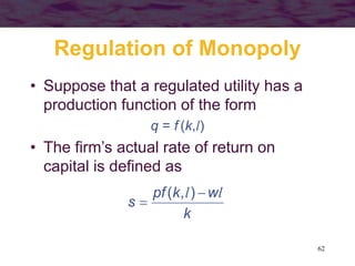
This document discusses models of monopoly and barriers to entry. It explains that a monopoly is a single supplier in a market and can choose any point on the demand curve to produce. Barriers to entry, which are the source of monopoly power, can be technical or legal. Technical barriers include economies of scale, unique knowledge, or ownership of resources. Legal barriers are created by patents, franchises, or lobbying. A monopolist maximizes profits where marginal revenue equals marginal cost and charges a price above marginal cost. The inverse elasticity rule relates the markup to demand elasticity. Monopolies can impact resource allocation, consumer surplus, and welfare losses compared to competition.

1. 1
Chapter 13
MODELS OF MONOPOLY
Copyright ©2005 by South-Western, a division of Thomson Learning. All rights reserved.

2. 2
Monopoly
• A monopoly is a single supplier to a
market
• This firm may choose to produce at any
point on the market demand curve

3. 3
Barriers to Entry
• The reason a monopoly exists is that
other firms find it unprofitable or
impossible to enter the market
• Barriers to entry are the source of all
monopoly power
– there are two general types of barriers to
entry
• technical barriers
• legal barriers

4. 4
Technical Barriers to Entry
• The production of a good may exhibit
decreasing marginal and average costs
over a wide range of output levels
– in this situation, relatively large-scale firms
are low-cost producers
• firms may find it profitable to drive others out of
the industry by cutting prices
• this situation is known as natural monopoly
• once the monopoly is established, entry of new
firms will be difficult

5. 5
Technical Barriers to Entry
• Another technical basis of monopoly is
special knowledge of a low-cost
productive technique
– it may be difficult to keep this knowledge
out of the hands of other firms
• Ownership of unique resources may
also be a lasting basis for maintaining a
monopoly

6. 6
Legal Barriers to Entry
• Many pure monopolies are created as a
matter of law
– with a patent, the basic technology for a
product is assigned to one firm
– the government may also award a firm an
exclusive franchise to serve a market

7. 7
Creation of Barriers to Entry
• Some barriers to entry result from actions
taken by the firm
– research and development of new products
or technologies
– purchase of unique resources
– lobbying efforts to gain monopoly power
• The attempt by a monopolist to erect
barriers to entry may involve real
resource costs

8. 8
Profit Maximization
• To maximize profits, a monopolist will
choose to produce that output level for
which marginal revenue is equal to
marginal cost
– marginal revenue is less than price because
the monopolist faces a downward-sloping
demand curve
• he must lower its price on all units to be sold if it
is to generate the extra demand for this unit

9. 9
Profit Maximization
• Since MR = MC at the profit-maximizing
output and P > MR for a monopolist, the
monopolist will set a price greater than
marginal cost

10. 10
C
Profits can be found in
the shaded rectangle
Profit Maximization
AC
MC
D
MR
Quantity
Price
Q*
The monopolist will maximize
profits where MR = MC
P* The firm will charge a price
of P*

11. 11
The Inverse Elasticity Rule
• The gap between a firm’s price and its
marginal cost is inversely related to the
price elasticity of demand facing the firm
PQeP
MCP
,
1


where eQ,P is the elasticity of demand
for the entire market

12. 12
The Inverse Elasticity Rule
• Two general conclusions about monopoly
pricing can be drawn:
– a monopoly will choose to operate only in
regions where the market demand curve is
elastic
• eQ,P < -1
– the firm’s “markup” over marginal cost
depends inversely on the elasticity of market
demand

13. 13
Monopoly Profits
• Monopoly profits will be positive as long
as P > AC
• Monopoly profits can continue into the
long run because entry is not possible
– some economists refer to the profits that a
monopoly earns in the long run as
monopoly rents
• the return to the factor that forms the basis of
the monopoly

14. 14
Monopoly Profits
• The size of monopoly profits in the long
run will depend on the relationship
between average costs and market
demand for the product

15. 15
Monopoly Profits
Quantity
Price
MC
AC
MR
D
Quantity
Price
MC
AC
MR
D
Positive profits Zero profit
P* P*=AC
C
Q* Q*

16. 16
No Monopoly Supply Curve
• With a fixed market demand curve, the
supply “curve” for a monopolist will only
be one point
– the price-output combination where MR =
MC
• If the demand curve shifts, the marginal
revenue curve shifts and a new profit-
maximizing output will be chosen

17. 17
Monopoly with Linear Demand
• Suppose that the market for frisbees
has a linear demand curve of the form
Q = 2,000 - 20P
or
P = 100 - Q/20
• The total costs of the frisbee producer
are given by
C(Q) = 0.05Q2 + 10,000

18. 18
Monopoly with Linear Demand
• To maximize profits, the monopolist
chooses the output for which MR = MC
• We need to find total revenue
TR = PQ = 100Q - Q2/20
• Therefore, marginal revenue is
MR = 100 - Q/10
while marginal cost is
MC = 0.01Q

19. 19
Monopoly with Linear Demand
• Thus, MR = MC where
100 - Q/10 = 0.01Q
Q* = 500 P* = 75
• At the profit-maximizing output,
C(Q) = 0.05(500)2 + 10,000 = 22,500
AC = 22,500/500 = 45
 = (P* - AC)Q = (75 - 45)500 = 15,000

20. 20
Monopoly with Linear Demand
• To see that the inverse elasticity rule
holds, we can calculate the elasticity of
demand at the monopoly’s profit-
maximizing level of output
3
500
75
20, 









Q
P
P
Q
e PQ

21. 21
Monopoly with Linear Demand
• The inverse elasticity rule specifies that
3
11
,


PQeP
MCP
• Since P* = 75 and MC = 50, this
relationship holds

22. 22
Monopoly and Resource
Allocation
• To evaluate the allocational effect of a
monopoly, we will use a perfectly
competitive, constant-cost industry as a
basis of comparison
– the industry’s long-run supply curve is
infinitely elastic with a price equal to both
marginal and average cost

23. 23
Monopoly and Resource
Allocation
Quantity
Price
MC=AC
D
MR
If this market was competitive, output would
be Q* and price would be P*
Q*
P*
Under a monopoly, output would be Q**
and price would rise to P**
Q**
P**

24. 24
Consumer surplus would fall
Producer surplus will rise
There is a deadweight
loss from monopoly
Monopoly and Resource
Allocation
Quantity
Price
MC=AC
D
MR
Q*Q**
P*
P** Consumer surplus falls by more
than producer surplus rises.

25. 25
Welfare Losses and Elasticity
• Assume that the constant marginal (and
average) costs for a monopolist are
given by c and that the compensated
demand curve has a constant elasticity:
Q = Pe
where e is the price elasticity of demand
(e < -1)

26. 26
Welfare Losses and Elasticity
• The competitive price in this market will
be
Pc = c
and the monopoly price is given by
e
c
Pm
1
1


27. 27
Welfare Losses and Elasticity
• The consumer surplus associated with
any price (P0) can be computed as



00
)(
P
e
P
dPPdPPQCS
11
1
0
1
0






e
P
e
P
CS
e
P
e

28. 28
Welfare Losses and Elasticity
• Therefore, under perfect competition
1
1



e
c
CS
e
c
1
1
1
1
















e
e
c
CS
e
m
and under monopoly

29. 29
Welfare Losses and Elasticity
• Taking the ratio of these two surplus
measures yields
1
1
1
1















e
c
m
e
CS
CS
• If e = -2, this ratio is ½
– consumer surplus under monopoly is half
what it is under perfect competition

30. 30
Welfare Losses and Elasticity
• Monopoly profits are given by
mmmmm Qc
e
c
cQQP















1
1
e
e
c
e
c
e
e
c
ee
m
1
1
1
1
1
1
1
1














































31. 31
Welfare Losses and Elasticity
• To find the transfer from consumer surplus
into monopoly profits we can divide
monopoly profits by the competitive
consumer surplus
e
e
c
m
e
e
e
e
e
CS


























 



11
1
11
1
• If e = -2, this ratio is ¼

32. 32
Monopoly and Product Quality
• The market power enjoyed by a monopoly
may be exercised along dimensions other
than the market price of its product
– type, quality, or diversity of goods
• Whether a monopoly will produce a
higher-quality or lower-quality good than
would be produced under competition
depends on demand and the firm’s costs

33. 33
Monopoly and Product Quality
• Suppose that consumers’ willingness to
pay for quality (X) is given by the inverse
demand function P(Q,X) where
P/Q < 0 and P/X > 0
• If costs are given by C(Q,X), the
monopoly will choose Q and X to
maximize
 = P(Q,X)Q - C(Q,X)

34. 34
Monopoly and Product Quality
• First-order conditions for a maximum are
0),( 





QC
Q
P
QXQP
Q
0





XC
X
P
Q
X
– MR = MC for output decisions
– Marginal revenue from increasing quality by
one unit is equal to the marginal cost of
making such an increase

35. 35
Monopoly and Product Quality
• The level of product quality that will be
opted for under competitive conditions is
the one that maximizes net social welfare
 
*
0
),(),(
Q
XQCdQXQPSW
• Maximizing with respect to X yields
 

 *
0
0),(
Q
XX CdQXQP
X
SW

36. 36
Monopoly and Product Quality
• The difference between the quality choice
of a competitive industry and the
monopolist is:
– the monopolist looks at the marginal
valuation of one more unit of quality
assuming that Q is at its profit-maximizing
level
– the competitve industry looks at the marginal
value of quality averaged across all output
levels

37. 37
Monopoly and Product Quality
• Even if a monopoly and a perfectly
competitive industry chose the same
output level, they might opt for diffferent
quality levels
– each is concerned with a different margin
in its decision making

38. 38
Price Discrimination
• A monopoly engages in price
discrimination if it is able to sell otherwise
identical units of output at different prices
• Whether a price discrimination strategy is
feasible depends on the inability of
buyers to practice arbitrage
– profit-seeking middlemen will destroy any
discriminatory pricing scheme if possible
• price discrimination becomes possible if resale is
costly

39. 39
Perfect Price Discrimination
• If each buyer can be separately
identified by the monopolist, it may be
possible to charge each buyer the
maximum price he would be willing to
pay for the good
– perfect or first-degree price discrimination
• extracts all consumer surplus
• no deadweight loss

40. 40
The monopolist will
continue this way until the
marginal buyer is no
longer willing to pay the
good’s marginal cost
Q1
P1
The first buyer pays P1 for Q1 units
Q2
P2 The second buyer pays P2 for Q2-Q1 units
Perfect Price Discrimination
Quantity
Price
D
Under perfect price discrimination, the monopolist
charges a different price to each buyer
MC

41. 41
Perfect Price Discrimination
• Recall the example of the frisbee
manufacturer
• If this monopolist wishes to practice
perfect price discrimination, he will want
to produce the quantity for which the
marginal buyer pays a price exactly
equal to the marginal cost

42. 42
Perfect Price Discrimination
• Therefore,
P = 100 - Q/20 = MC = 0.1Q
Q* = 666
• Total revenue and total costs will be
511,55
40
100)(
666
0
*
0
2
 
Q Q
QdQQPR
178,32000,1005.0)( 2
 QQc
• Profit is much larger (23,333 > 15,000)

43. 43
Market Separation
• Perfect price discrimination requires the
monopolist to know the demand function
for each potential buyer
• A less stringent requirement would be to
assume that the monopoly can separate its
buyers into a few identifiable markets
– can follow a different pricing policy in each
market
– third-degree price discrimination

44. 44
Market Separation
• All the monopolist needs to know in this
case is the price elasticities of demand
for each market
– set price according to the inverse elasticity
rule
• If the marginal cost is the same in all
markets,
)
1
1()
1
1(
j
j
i
i
e
P
e
P 

45. 45
Market Separation
• This implies that
)
1
1(
)
1
1(
i
j
j
i
e
e
P
P



• The profit-maximizing price will be
higher in markets where demand is less
elastic

46. 46
Market Separation
Quantity in Market 2Quantity in Market 1
Price
0
DD
MRMR
MCMC
Q2*
P2
Q1*
P1
If two markets are separate, maximum profits occur by
setting different prices in the two markets
The market with the less
elastic demand will be
charged the higher price

47. 47
Third-Degree Price
Discrimination
• Suppose that the demand curves in two
separated markets are given by
Q1 = 24 – P1
Q2 = 24 – 2P2
• Suppose that MC = 6
• Profit maximization requires that
MR1 = 24 – 2Q1 = 6 = MR2 = 12 – Q2

48. 48
Third-Degree Price
Discrimination
• Optimal choices and prices are
Q1 = 9 P1 = 15
Q2 = 6 P2 = 9
• Profits for the monopoly are
 = (P1 - 6)Q1 + (P2 - 6)Q2 = 81 + 18 = 99

49. 49
Third-Degree Price
Discrimination
• The allocational impact of this policy can be
evaluated by calculating the deadweight
losses in the two markets
– the competitive output would be 18 in market 1
and 12 in market 2
DW1 = 0.5(P1-MC)(18-Q1) = 0.5(15-6)(18-9) = 40.5
DW2 = 0.5(P2-MC)(12-Q2) = 0.5(9-6)(12-6) = 9

50. 50
Third-Degree Price
Discrimination
• If this monopoly was to pursue a single-
price policy, it would use the demand
function
Q = Q1 + Q2 = 48 – 3P
• So marginal revenue would be
MR = 16 – 2Q/3
• Profit-maximization occurs where
Q = 15 P = 11

51. 51
Third-Degree Price
Discrimination
• The deadweight loss is smaller with one
price than with two:
DW = 0.5(P-MC)(30-Q) = 0.5(11-6)(15) = 37.5

52. 52
Two-Part Tariffs
• A linear two-part tariff occurs when
buyers must pay a fixed fee for the right
to consume a good and a uniform price
for each unit consumed
T(q) = a + pq
• The monopolist’s goal is to choose a
and p to maximize profits, given the
demand for the product

53. 53
Two-Part Tariffs
• Because the average price paid by any
demander is
p’ = T/q = a/q + p
this tariff is only feasible if those who
pay low average prices (those for whom
q is large) cannot resell the good to
those who must pay high average
prices (those for whom q is small)

54. 54
Two-Part Tariffs
• One feasible approach for profit
maximization would be for the firm to set
p = MC and then set a equal to the
consumer surplus of the least eager
buyer
– this might not be the most profitable
approach
– in general, optimal pricing schedules will
depend on a variety of contingencies

55. 55
Two-Part Tariffs
• Suppose there are two different buyers
with the demand functions
q1 = 24 - p1
q2 = 24 - 2p2
• If MC = 6, one way for the monopolist to
implement a two-part tariff would be to
set p1 = p2 = MC = 6
q1 = 18 q2 = 12

56. 56
Two-Part Tariffs
• With this marginal price, demander 2
obtains consumer surplus of 36
– this would be the maximum entry fee that
can be charged without causing this buyer
to leave the market
• This means that the two-part tariff in this
case would be
T(q) = 36 + 6q

57. 57
Regulation of Monopoly
• Natural monopolies such as the utility,
communications, and transportation
industries are highly regulated in many
countries

58. 58
Regulation of Monopoly
• Many economists believe that it is
important for the prices of regulated
monopolies to reflect marginal costs of
production accurately
• An enforced policy of marginal cost
pricing will cause a natural monopoly to
operate at a loss
– natural monopolies exhibit declining
average costs over a wide range of output

59. 59
Regulation of Monopoly
Quantity
Price
D
MR
AC
MC
Because natural monopolies exhibit
decreasing costs, MC falls below AC
C1
P1
Q1
An unregulated monopoly will
maximize profit at Q1 and P1
C2
P2
Q2
If regulators force the
monopoly to charge a
price of P2, the firm will
suffer a loss because
P2 < C2

60. 60
cover the losses on the sales to
low-price customers
The profits on the sales to high-
price customers are enough to
Regulation of Monopoly
Quantity
Price
D
AC
MC
Suppose that the regulatory commission allows the
monopoly to charge a price of P1 to some users
P1
Q1
C1
Other users are offered the lower price
of P2
P2
Q2
C2

61. 61
Regulation of Monopoly
• Another approach followed in many
regulatory situations is to allow the
monopoly to charge a price above
marginal cost that is sufficient to earn a
“fair” rate of return on investment
– if this rate of return is greater than that
which would occur in a competitive market,
there is an incentive to use relatively more
capital than would truly minimize costs

62. 62
Regulation of Monopoly
• Suppose that a regulated utility has a
production function of the form
q = f (k,l)
• The firm’s actual rate of return on
capital is defined as
k
wkpf
s
ll 

),(

63. 63
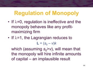
Regulation of Monopoly
• Suppose that s is constrained by
regulation to be equal to s0, then the
firm’s problem is to maximize profits
 = pf (k,l) – wl – vk
subject to this constraint
• The Lagrangian for this problem is
L = pf (k,l) – wl – vk + [wl + s0k – pf (k,l)]

64. 64
Regulation of Monopoly
• If =0, regulation is ineffective and the
monopoly behaves like any profit-
maximizing firm
• If =1, the Lagrangian reduces to
L = (s0 – v)k
which (assuming s0>v), will mean that
the monopoly will hire infinite amounts
of capital – an implausible result

65. 65
Regulation of Monopoly
• Therefore, 0<<1 and the first-order
conditions for a maximum are:
0)( 


ll
l
pfwwpf
L
0)( 0 


kk pfsvpf
k
L
0),(0 


ll kpfsw
L

66. 66
Regulation of Monopoly
• Because s0>v and <1, this means that
pfk < v
• The firm will hire more capital than it
would under unregulated conditions
– it will also achieve a lower marginal
productivity of capital

67. 67
Dynamic Views of Monopoly
• Some economists have stressed the
beneficial role that monopoly profits can
play in the process of economic
development
– these profits provide funds that can be
invested in research and development
– the possibility of attaining or maintaining a
monopoly position provides an incentive to
keep one step ahead of potential competitors

68. 68
Important Points to Note:
• The most profitable level of output for
the monopolist is the one for which
marginal revenue is equal to marginal
cost
– at this output level, price will exceed
marginal cost
– the profitability of the monopolist will
depend on the relationship between price
and average cost

69. 69
Important Points to Note:
• Relative to perfect competition,
monopoly involves a loss of consumer
surplus for demanders
– some of this is transferred into monopoly
profits, whereas some of the loss in
consumer surplus represents a
deadweight loss of overall economic
welfare
– it is a sign of Pareto inefficiency

70. 70
Important Points to Note:
• Monopolies may opt for different levels
of quality than would perfectly
competitive firms
• Durable good monopolists may be
constrained by markets for used goods

71. 71
Important Points to Note:
• A monopoly may be able to increase its
profits further through price
discrimination – charging different
prices to different categories of buyers
– the ability of the monopoly to practice
price discrimination depends on its ability
to prevent arbitrage among buyers

72. 72
Important Points to Note:
• Governments often choose to regulate
natural monopolies (firms with
diminishing average costs over a broad
range of output levels)
– the type of regulatory mechanisms
adopted can affect the behavior of the
regulated firm