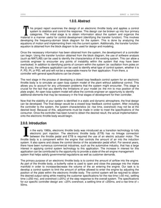
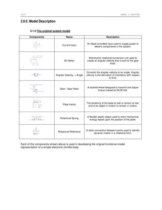
This document summarizes the design process for developing a closed-loop feedback control system for an electronic throttle body. It involves:
1) Modeling the system to obtain the transfer function.
2) Analyzing the transfer function using MATLAB to determine if the system is stable or oscillatory.
3) Simulating an open-loop model to account for real-world non-idealities.
4) Designing a PD controller to meet specifications and stabilize the oscillatory system. The controller is tuned using MATLAB simulations.
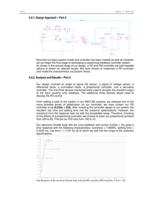
5) Implementing the designed controller in a closed-loop system model in System Vision software.
![2006 ERNST & SAPUTRA
5. Simulate the controller while apply a sweep of gain values.
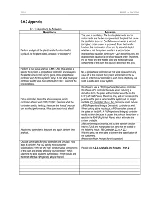
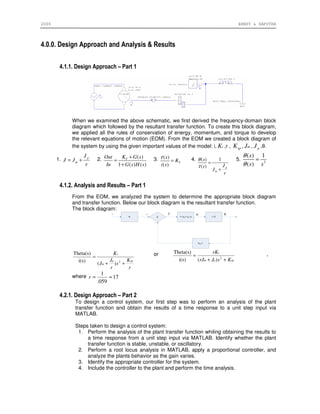
4.2.2. Analysis and Results – Part 2
We performed an analysis of the plant transfer function and a time response to a unit
step input by using MATLAB.
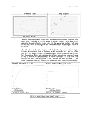
The root locus shown above demonstrates how the system is expected to design
when the gain is varied. In other words, if you were to include a proportional controller
and change the K value of it, you will notice how the system changes. According to our
representation of the system, the poles will never leave the jω axis and therefore will
remain oscillatory regards of the proportional gain that is included into the system. This
can be seen in the image to the right, where the time response continues to oscillate
around 0.5. This response identifies a P controller as not the ideal controller this
application.
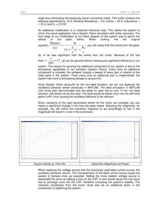
It can be seen in the time response that the plant is oscillatory. The throttle plate
inertia and dc motor inertia are the two components of the plant that cause the
oscillation to occur. Oscillation occurs when a second (or higher) order system is
introduced into the transfer function. From the transfer function, the combination of Jm
and Jp are what determine whether or not the system results in a second order
characteristic equation. When (Jm + Jp/r) becomes zero, the characteristic equation is
no longer second order. Therefore, the dc motor and the throttle plate are the two
physical components of the plant that cause it to behave this way.
Applying a proportional controller will not work because for any value of ‘k’ the poles of
the system will remain on the jω axis. In order for our controller to work more
effectively, we need to add a zero to our system.
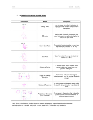
We chose to use a PD (Proportional Derivative) controller. We chose a PD controller
because when including a derivative term, the poles will be located would be on the
LHP (Left Half Plane). Therefore, they will not remain on the jω axis as the gain is
varied and the system will no longer oscillate. PD Controller: (KDs + KP). Someone
could include a PID (Proportional Integral Derivative) controller as well. When looking
at the root locus, a PID controller places all the poles on the LHP. A PI (Proportional
Integral) controller would not work because it causes the poles of the system to result
in the RHP (Right Half Plane) which will make the system unstable.
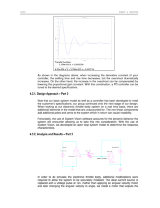
After performing an analysis, we put the transfer function into MATLAB and
manipulated our zero that we added the following to our result: PD Controller: (0.233*s
+ 233). With this zero included into our MATLAB simulation, we were able to achieve
the specification of the customers.
Plant Transfer Function Analysis: Time Response to a Unit Step Input:
sys=tf([-.0187],[(-4.0295*10^-6) 0 -.003182]);
rltool(sys)
(additional option with rltool)](https://image.slidesharecdn.com/47e515ec-ab65-4a04-9c38-b5153a0ff2aa-161205045939/85/Unity-Feedback-PD-Controller-Design-for-an-Electronic-Throttle-Body-6-320.jpg)