Download as PDF, PPTX


![Confidence Intervals
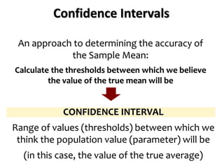
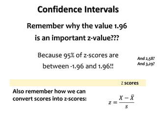
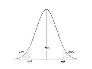
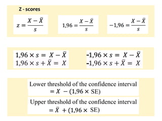
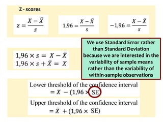
If we know that our limits will be -1.96 and 1.96, in z-
scores, what are the corresponding scores in values
of our data?
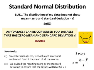
[It is the inverse of how to calculate the Z score]
To find this, let's put z back into the equation
Z score](https://image.slidesharecdn.com/probability1-241029005155-d03efb9e/85/Probability-and-Statistical-Inference-2024-66-320.jpg)
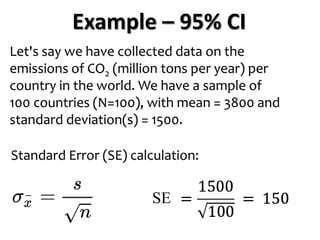
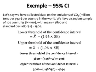
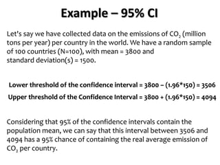
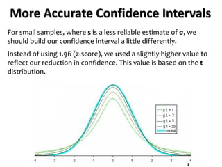


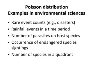

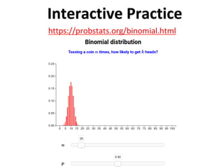
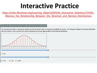
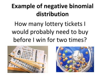

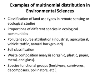


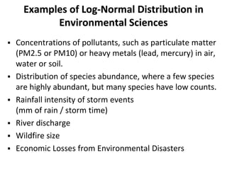
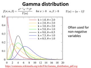
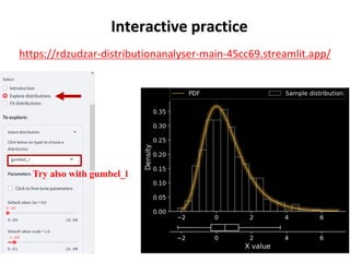
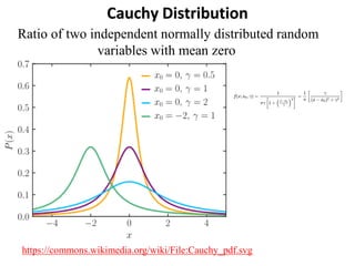
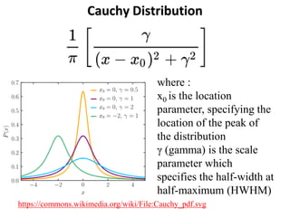
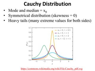

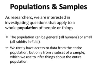
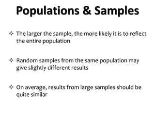
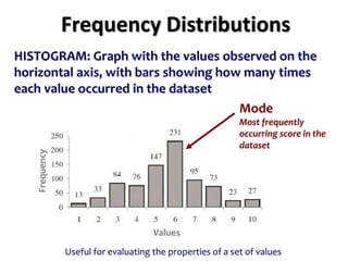
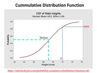
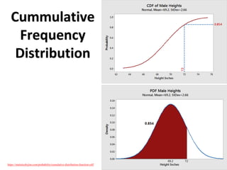
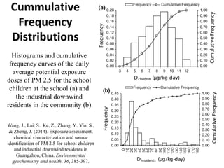
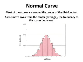
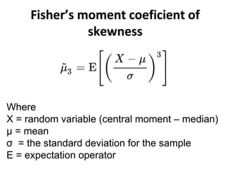
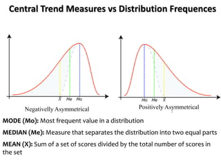
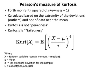
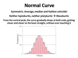
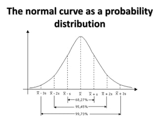
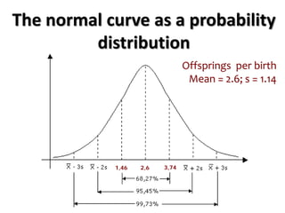
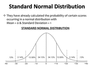
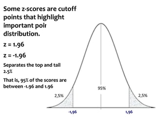
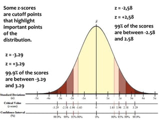
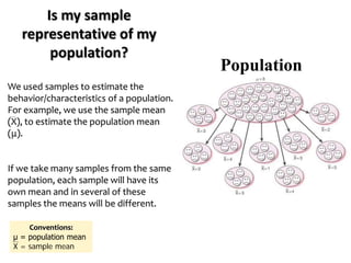
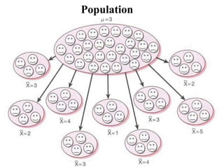
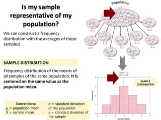
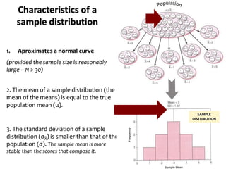
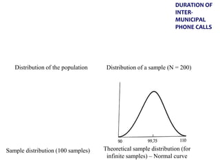
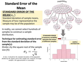
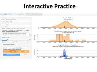
The document outlines key concepts in environmental data analysis, focusing on probability distributions, statistical inference, and confidence intervals. It discusses the importance of populations and samples, the normal curve, and various measures used in statistics such as mean, median, mode, and standard error. Practical applications using R for data analysis are included, alongside the significance of estimating population parameters from sample data.


![[DL輪読会]Attentive neural processes](https://cdn.slidesharecdn.com/ss_thumbnails/attentiveneuralprocesses-181225051145-thumbnail.jpg?width=640&height=640&fit=bounds)