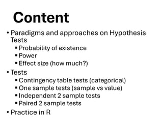
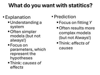
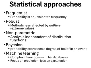
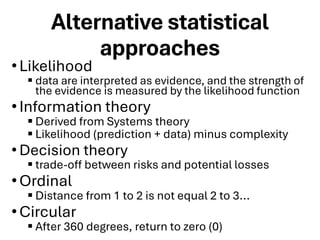
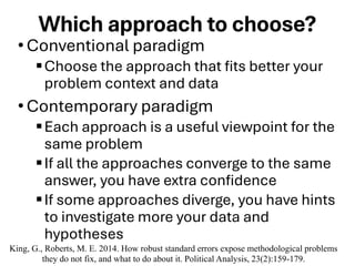
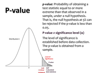
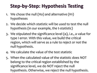
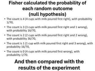
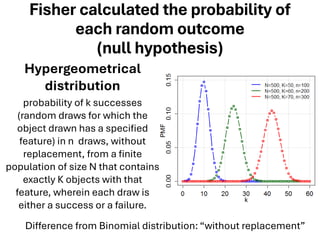
The document explores various statistical methodologies for hypothesis testing, focusing on different paradigms including frequentist, Bayesian, and machine learning approaches. It covers the construction and testing of null and alternative hypotheses, types of statistical errors, p-values, effect sizes, and how to interpret results in environmental data analysis. Additionally, the content includes practical applications of statistical tests using R programming to analyze various data scenarios.

1. Environmental Data Analysis:
Hypothesis testing
Vitor Vieira Vasconcelos
João Marcelo Borovina Josko
Federal University of ABC (UFABC)
São Bernardo do Campo-SP, Brazil
October 2024

2. Content
• Paradigms and approaches on Hypothesis
Tests
▪Probability of existence
▪Power
▪Effect size (how much?)
• Tests
▪Contingency table tests (categorical)
▪One sample tests (sample vs value)
▪Independent 2 sample tests
▪Paired 2 sample tests
• Practice in R

3. What do you want with statitics?
•Explanation
▪Understanding a
system
▪Often simpler
models (but not
always!)
▪Focus on
parameters, which
represent the
hypotheses
▪Think: causes of
effects
• Prediction
▪Focus on fitting Y
▪Often results more
complex models
(but not Always!)
▪Think: effects of
causes

4. Statistical approaches
• Frequentist
▪ Probability is equivalent to frequency
• Robust
▪ Methods less affected by outliers
(extreme values)
• Non-parametric
▪Analysis independent of distribution
functions
• Bayesian
▪ probability expresses a degree of belief in an event
• Machine learning
▪ Complex interactions with big databases
▪ Focus on prediction, less on explanation

5. Alternative statistical
approaches
•Likelihood
▪ data are interpreted as evidence, and the strength of
the evidence is measured by the likelihood function
•Information theory
▪ Derived from Systems theory
▪ Likelihood (prediction + data) minus complexity
•Decision theory
▪ trade-off between risks and potential losses
•Ordinal
▪ Distance from 1 to 2 is not equal 2 to 3...
•Circular
▪ After 360 degrees, return to zero (0)

6. Which approach to choose?
•Conventional paradigm
▪Choose the approach that fits better your
problem context and data
•Contemporary paradigm
▪Each approach is a useful viewpoint for the
same problem
▪If all the approaches converge to the same
answer, you have extra confidence
▪If some approaches diverge, you have hints
to investigate more your data and
hypotheses
King, G., Roberts, M. E. 2014. How robust standard errors expose methodological problems
they do not fix, and what to do about it. Political Analysis, 23(2):159-179.

7. Fequentist approach
Null and Alternative Hypotheses

8. To test the significance of a relationship in a
model, we establish a (null) hypothesis that no
relationship exists in the population.
HYPOTHESES
- Experimental hypothesis (or alternative hypothesis)
(H1) → It usually corresponds to a "prediction" made by
the researcher (There is a relationship between variables in the
population)
Null hypothesis (H0) → The predicted effect does not
exist
(There is a relationship between variables in the population)
It has become a convention in statistical analysis to start the study with the
null hypothesis test.

10. To confirm or reject our hypotheses:
We calculate the probability that the observed
effect (in our case, the relationship) occurred by
chance: As the probability of "chance" decreases,
we confirm that the experimental hypothesis is
correct and that the null hypothesis can be
rejected.

11. And when can we consider that a result is genuine, that
is, it is not the result of chance?
There is always a risk that we consider an
effect true, when, in fact, it is not (TYPE I
ERROR). For Ronald Fisher, only when the
probability of something happening by
chance is equal to or less than 5% (<0.05),
can we accept that it is an outcome
statistically significant.
The value of the probability of making a
type I error in a hypothesis test is known as
LEVEL OF SIGNIFICANCE and is represented
by the letter α
The most commonly used significance levels are 5%, 1% and 0.1%

12. ▪ To establish whether a model (in this case, the
relationship between two variables) is a reasonable
representation of what's going on, we usually calculate a
TEST STATISTIC.
▪ It is a statistic that has known properties, we already
know how often different values of this statistic occur.
▪ We know their distributions and this allows us, once we
have calculated the test statistic, to calculate a value as
large as the one we have. If we have a test statistic of 100,
for example, we could then calculate the probability of
getting such a large value.
Test Statistics

13. Test Statistics
There are several statistical tests (t, F...).
However, most of them represent the following:
The exact shape of this equation changes from test to
test.
If our model is good, we expect the variance it explains
to be greater than the variance it can't explain.
𝑻𝒆𝒔𝒕 𝒔𝒕𝒂𝒕𝒊𝒔𝒕𝒊𝒄 =
𝑉𝑎𝑟𝑖𝑎𝑛𝑐𝑒 𝑒𝑥𝑝𝑙𝑎𝑖𝑛𝑒𝑑 𝑏𝑦 𝑡ℎ𝑒 𝑚𝑜𝑑𝑒𝑙
𝑉𝑎𝑟𝑖𝑎𝑛𝑐𝑒 𝑛𝑜𝑡 𝑒𝑥𝑝𝑙𝑎𝑖𝑛𝑒𝑑 𝑏𝑦 𝑡ℎ𝑒 𝑚𝑜𝑑𝑒𝑙

14. The higher the test statistic, the less likely it is that our
results are the result of chance.
When this probability drops below 0.05 (Fisher's
criterion), we accept this as enough confidence to
assume that the test statistic is so large because our
model accounts for enough variation to reflect what is
actually happening in the real world (the population)
Test Statistics

15. The higher the test statistic, the less likely it is that our
results are the result of chance.
That is,
We reject our null hypothesis and accept our
experimental hypothesis
Test Statistics

16. Null hypothesis Experimental Hypothesis
Test Statistics
REJECTED!

19. Jawlik, A. A. (2016). Statistics from A to Z: Confusing Concepts Clarified. John Wiley & Sons.

20. Jawlik, A. A. (2016). Statistics from A to Z: Confusing Concepts Clarified. John Wiley & Sons.
Experimental hypothesis:
there are unicorns in São Bernardo do Campo
Null hypothesis:
there are no unicorns in São Bernardo do Campo
We cannot reject the null hypothesis that there are no
unicorns in São Bernardo do Campo

21. Directional Hypothesis: “When one variable
increases, the other variable also increases”
→ ONE-SIDED (tailed) HYPOTHESIS TESTING
Non-Directional Hypothesis: “When one
variable increases, the other variable also
increases, or decreases”
→ BILATERAL (2 tailed) HYPOTHESIS TESTING
Unilateral and Bilateral Tests

22. 𝛼
ൗ
𝛼
2
ൗ
𝛼
2
Reject the null hypothesis if
t calculated < t threshold
Reject the null hypothesis if
|t calculated| > t threshold
https://www.geeksforgeeks.org/difference-between-one-tailed-and-two-tailed-tests/
Rejection Regions
Reject the null hypothesis if
t calculated > t threshold
𝛼

23. Rejection Regions
https://datatab.net/tutorial/one-sample-t-test

24. Example of tables of critical values
of t distribution

25. P-value
p-value: Probability of obtaining a
test statistic equal to or more
extreme than that observed in a
sample, under a null hypothesis.
That is, the null hypothesis at 5% can
be rejected if the p-value is less than
0.05.
P-value ≠ significance level (α)
The level of significance is
established before data collection.
The p-value is obtained from a
sample.
1,64
t Critical
2,87
t calculated
(test statistics)
Level of
Significance
P-value
Distribution t
Unilateral

27. 1. We chose the null (Ho) and alternative (H1)
hypotheses
2. We decide which statistic will be used to test the null
hypothesis (in our example, the t-statistic)
3. We stipulated the significance level (α), i.e., a value for
type I error. With this value, we build the critical
region, which will serve as a rule to reject or not the
null hypothesis.
4. We calculate the value of the test statistic
5. When the calculated value of the statistic does NOT
belong to the critical region established by the
significance level, we do NOT reject the null
hypothesis. Otherwise, we reject the null hypothesis.
Step-by-Step: Hypothesis Testing

28. Fisher’s exact test
A lady in a party told Ronald Fisher
“I can tell whether the milk is poured
first, and the tea is added next, or
whether the tea is poured first, and
the milk is added to the tea.”

29. Plan a number of trials
• Arrange a number of
cups
▪ Fisher proposed 8 cups
▪ Half with tea first
▪ Half with milk first
▪ Present them in random
order
• Then have the lady taste
them and make her
decisions

30. Fisher calculated the probability of
each random outcome
(null hypothesis)
• The count is 4 (4 cups with milk poured first right), with probability
1/70,
• The count is 3 (3 cups with milk poured first right and 1 wrong),
with probability 16/70,
• The count is 2 (2 cups with milk poured first right and 2 wrong),
with probability 36/70,
• The count is 1 (1 cup with milk poured first right and 3 wrong), with
probability 16/70,
• The count is 0 (4 cups with milk poured first wrong), with
probability 1/70.
And then compared with the
results of the experiment

31. Fisher calculated the probability of
each random outcome
(null hypothesis)
Hypergeometrical
distribution
probability of k successes
(random draws for which the
object drawn has a specified
feature) in n draws, without
replacement, from a finite
population of size N that contains
exactly K objects with that
feature, wherein each draw is
either a success or a failure.
Difference from Binomial distribution: “without replacement”

32. Practice in R

33. χ 2 (Chi-square) distribution
sum of the squares of k independent standard
normal random variables

34. χ 2 (Chi-square) test
Analysis of Contingency Tables
(two categorical variables)
Tests whether two categorical variables
(two dimensions of the contingency table)
are independent in influencing the test statistic
(values within the table)
Classification
A B C
Classification
R 5 8 7
S 7 3 8
T 6 8 7
Null hypothesis: Are these numbers randomly distributed ?

35. Practice in R

36. History of continuous variables tests
1. Z-test
• Comparison of means of two samples using normal z-
score distribution
2. t-test
• Uses t-distribution instead of normal distribution
• Assumptions = variance is equal between samples
• f-test: are variances equal among samples?
3. t-test with Welch correction
• Adjust for unequal variance between samples
4. Permutational t-test
• Does not require t or normal distribution

37. t-test
Uses t distribution
https://datatab.net/tutorial/t-test

38. Single sample t-test
determine if a single group is significantly different from a population value
t distribution
https://www.statstest.com/single-sample-t-test/

39. Single sample t-test
https://datatab.net/tutorial/t-test

40. https://www.statstest.com/independent-samples-t-test/
Independent samples
t-test

41. Independent samples t-test
https://datatab.net/tutorial/t-test

42. Paired samples t-test

43. Paired samples
t-test
https://datatab.net/tutorial/t-test

44. F-test
Are variances different among two samples?
Variance of group A
Variance of group B

45. F Distribution
d1 and d2 are the
degrees of freedom
of each sample

46. Examples of questions regarding variance
difference in Environmental Sciences
• Is weather (rainfall or temperature) becoming
more variable or not, comparing to a previous
moment in the past?
• Did the construction of a dam stabilize the
flow variation downstream of a river?
• Is variation of a water quality parameter (such
as nutrient concentration) different between
tropical or temperate lakes?
• Is annual variation of energy production by
solar power different than by wind?

47. Practice in R

48. Type II Error (beta)
Probability of failing to reject
the null hypothesis when it’s
actually false

49. True state of nature
H0 is true Ha is true
Conclusion
Support H0 /
Reject Ha
Correct
conclusion
Type II Error
Support Ha /
Reject H0
Type I Error Correct
conclusion

50. True state of nature
H0 is true Ha is true
Conclusion
Support H0 /
Reject Ha
Correct
conclusion
True
negative
Type II Error
False
negative
Support Ha /
Reject H0
Type I Error
False
positive
Correct
conclusion
True positive

51. https://www.scribbr.com/statistics/type-i-and-type-ii-errors/

52. True state of nature
H0 is true Ha is true
Conclusion
Support H0 /
Reject Ha
Correct
conclusion
True
negative
Probability = 1- α
Type II Error
False
negative
Probability = β
Support Ha /
Reject H0
Type I Error
False
positive
Probability = α
Correct
conclusion
True positive
Probability = 1- β

53. Statistical Power
Statistical power is the probability of
finding an effect when the effect is real.
So a statistical power of 80% means
that out of 100 tests where variations
are different, 20 tests will conclude
that variations are the same and no
effect exists.

54. Power is directly related to sample size
Arnoldo, T., & Víctor, C. V. (2015). Effect size, confidence intervals and statistical power in psychological research.
Psychology in Russia: State of the art, 8(3), 27-46.
Power of 2 independent groups, each one size N
Power
N, size of each group

55. True state of nature
H0 is true Ha is true
Conclusion
Support H0 /
Reject Ha
Correct
conclusion
True
negative
Probability = 1- α
Type II Error
False
negative
Probability = β
Support Ha /
Reject H0
Type I Error
False
positive
Probability = α
Correct
conclusion
True positive
Probability = 1- β
Power

56. https://www.qualitygurus.com/type-i-and-type-ii-errors-explained/

57. Effect
size
Difference in
the mean of
the
distribution
function
between two
groups
Arnoldo, T., & Víctor, C. V.
(2015). Effect size,
confidence intervals and
statistical power in
psychological research.
Psychology in Russia: State
of the art, 8(3), 27-46.

58. Cramér’s V Effect size
• Effect size between categorical variables
• Changes from
▪ 0 = two categorical variables are not associated
▪ 1 = two categorical variables are totally associated

59. Cramér’s V Effect size
• Changes from
▪ 0 = two categorical variables are not associated
▪ 1 = two categorical variables are totally associated
Degrees of
freedom
Small Medium Large
1 0.10 0.30 0.50
2 0.07 0.21 0.35
3 0.06 0.17 0.29
4 0.05 0.15 0.25
5 0.04 0.13 0.22
https://www.statology.org/interpret-cramers-v/

60. Cohen effect size
𝑑 =
ത
𝑋 𝑒𝑥𝑝𝑒𝑟𝑖𝑚𝑒𝑛𝑡 − ത
𝑋 𝑐𝑜𝑛𝑡𝑟𝑜𝑙
𝑆𝐷 𝑐𝑜𝑚𝑏𝑖𝑛𝑒𝑑
Cohen, J. (1988). Statistical power analysis for the behavioral
sciences (2nd ed.). Hillsdale, NJ: Lawrence Earlbaum
Associates.

61. Cohen's d effect size Interpretation
d=.0 to .19 Trivial effect
d= .20 Small effect
d= .50 Medium effect
d=.80 or higher Large effect
Cohen effect size
Cohen, J. (1992a). A power primer. Psychological Bulletin, 112(1), 155. doi:10.1037/0033-
2909. 112.1.155
Cohen, J. (1992b). Statistical power analysis. Current Directions in Psychological
Science, 1(3), 98-101.

62. Null
hypothesis
Alternate
hypothesis
https://vwo.com/tools/ab-test-significance-calculator/

63. Practice in R

64. Ranking non-parametric versions
of tests
• Compare medians
instead of means
• Advantages
▪Doesn’t assume a
probability distribution
▪Less affected by extreme
values
• Disadvantage
▪Less certainty than
parametric tests (higher
p-values)
Variable
5
3
4
8
10
2
7
5
Ranking
4,5
2
3
7
8
1
6
4,5

65. Equivalent versions
Parametric Non Parametric
One sample t test Wilcoxon signed-rank test
(one sample)
Two independent samples
t-tests
Wilcoxon signed-rank test
(two samples)
Paired t-test Mann-Whitney U test

66. Effect size for Non Parametric Tests
Vargha and
Delaney’s A
Effect size
> 0.34 Large
0.34-0.29 Medium
≤ 29 Small
Vargha, A. and H.D. Delaney. A Critique and Improvement of the CL Common Language
Effect Size Statistics of McGraw and Wong. 2000. Journal of Educational and Behavioral
Statistics 25(2):101–132.

67. Practice in R

68. •Parametric methods
▪Assumes distribution
of statistics under
null hypothesis
•Non-parametric
permutation tests
▪Use data resampling
to find the
distribution under
null hypothesis

69. Practice in R