The document discusses the Matlab PDE Toolbox. It can be used to solve partial differential equations (PDEs) in 2D and 3D using finite element analysis. The toolbox allows users to specify geometries, boundary conditions, equations and solve static, time dependent and other types of PDE problems. An example problem describing heat transfer in a circular object is presented and solved using the pdepe solver function. Plots of the temperature distribution over time and distance are generated. Applications of the toolbox include electrostatics, structural mechanics, heat transfer and more.

1. Matlab
PDE Tool Box
GROUP 6
1

2. Outline
Introduction
Why we need it
PDE functions
Example problem
Solution of the problem
Code of the solution
Application
2

3. Introduction 14-01-07-031
What is PDE?
In mathematics, a partial differential equation (PDE) is a differential equation that contains
unknown multivariable functions and their partial derivatives. (A special case is ordinary
differential equations (ODEs), which deal with functions of a single variable and their
derivatives.)
PDEs are used to formulate problems involving functions of several variables, and are either
solved by hand, or used to create a relevant computer model.
3

4. Introduction
PDE Toolbox
Partial Differential Equation Toolbox™ provides functions for solving partial differential
equations (PDEs) in 2-D, 3-D, and time using finite element analysis.
It enables to specify and mesh 2-D and 3-D geometries and formulate boundary conditions and
equations.
It can solve static, time domain, frequency domain, and eigenvalue problems over the domain of
the geometry
4

5. Introduction: Opening PDE toolbox
Using the Apps Tab
On the MATLAB Toolstrip, click the Apps tab.
On the Apps tab, click the down arrow at the end of the Apps section.
Under Math, Statistics and Optimization, click the PDE button.
5

6. Introduction: Opening PDE toolbox
Using commands
To open a blank PDE app window, type pdetool in the MATLAB Command Window.
To open the PDE app with a circle already drawn in it, type pdecirc in the MATLAB Command
Window.
To open the PDE app with an ellipse already drawn in it, type pdeellip in the MATLAB Command
Window.
To open the PDE app with a rectangle already drawn in it, type pderect in the MATLAB
Command Window.
To open the PDE app with a polygon already drawn in it, type pdepoly in the MATLAB Command
Window.
6

7. Why do we need it 14-01-07-035
Time dependent pde
Changing with Space
7

8. PDE Setup
Create or import the geometry for your problem, a 2-D or 3-D region.
Set boundary conditions on the outer edges or faces of the geometry.
Specify the PDE coefficients.
Specify initial conditions.
Create a finite element mesh of the geometry.
Call the solver.
8

9. PDE Functions
Sol=pdepe(m, pdefun, icfun, bcfun, xmesh, tspan)
9

10. Problem 14-01-07-050
10
At center
𝑑𝑇
𝑑𝑟
=0
temperature convection
−
𝑑𝑇
𝑑𝑟
=
ℎ
𝑘
𝑇 − 𝑇α
So for radius r the PDE is
𝑑𝑇
𝑑𝑡
= α
1
𝑟2
𝑑
𝑑𝑟
(
𝑟2 𝑑𝑇
𝑑𝑟
)

11. Problem 14-01-07-046
initial condition
T₀= 5ᵒC
Boundary condition
@r=0
𝑑𝑇
𝑑𝑟
= 0
@r=0.05 −
𝑑𝑇
𝑑𝑟
=
ℎ
𝑘
𝑇 − 𝑇α
11

12. Solution
PDE form of MATLAB
C
𝑑𝑢
𝑑𝑡
= 𝑥−𝑚 𝑑𝑢
𝑑𝑥
(𝑥 𝑚 𝑓 𝑥, 𝑡, 𝑢,
𝑑𝑢
𝑑𝑥
+ 𝑠
Our equation is
1
α
𝑑𝑇
𝑑𝑡
= 𝑟−2 𝑑
𝑑𝑟
𝑟2 𝑑𝑇
𝑑𝑟
+ 0 𝑜𝑟
1
α
𝑑𝑢
𝑑𝑥
= 𝑟−2 𝑑
𝑑𝑥
𝑥2 𝑑𝑢
𝑑𝑥
+ 0
12

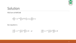
13. Code 14-01-07-045
function FLASH
m=2;
xmesh=linspace(0, 0.05, 20);
tspan=linspace(0,28800,32);
sol=pdepe(m, @pdefun, @icfun, @bcfun, xmesh,
tspan);
U=sol(:,:,1);
13
Function [c,f,s]=pdefun[x,t,u,DuDx]
C=1/ α;
F=DuDx;
S=0
Function u0=icfun(x)
u0=5;

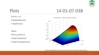
14. code
Function [pl, ql, pr, qr]=pdebc(xl, ul, xr, ur, t)
pl=0;
ql=1;
Because matlab uses
P+qf=0
On left (center)
𝑑𝑇
𝑑𝑥
= 0 so, 0+1
𝑑𝑇
𝑑𝑥
=0
14

15. Plots 14-01-07-038
Surf (x, t, u)
X label(‘distance’)
Y label(‘time’)
Figure
Plot (x,u,(end,:))
X label (‘distance’)
Y label (‘temperature’)
15
Picture is downloaded from internet. But the actual curve for this equation will look like this.

16. Applications
 Electrostatics and Magneto statics
 Structural Mechanics
 DC Conduction and Elliptic Problems
 Heat Transfer and Diffusion
16

17. 17
This presentation is made with the help of this video
https://www.youtube.com/watch?v=ri_1nxwupb8&t=596s