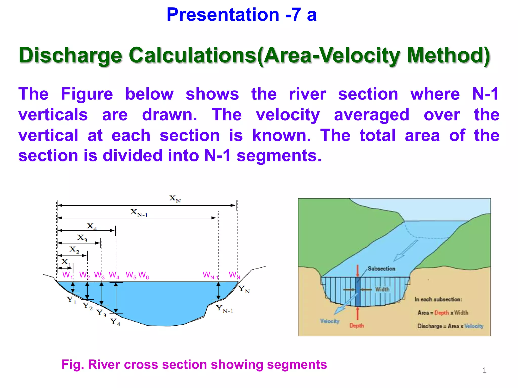
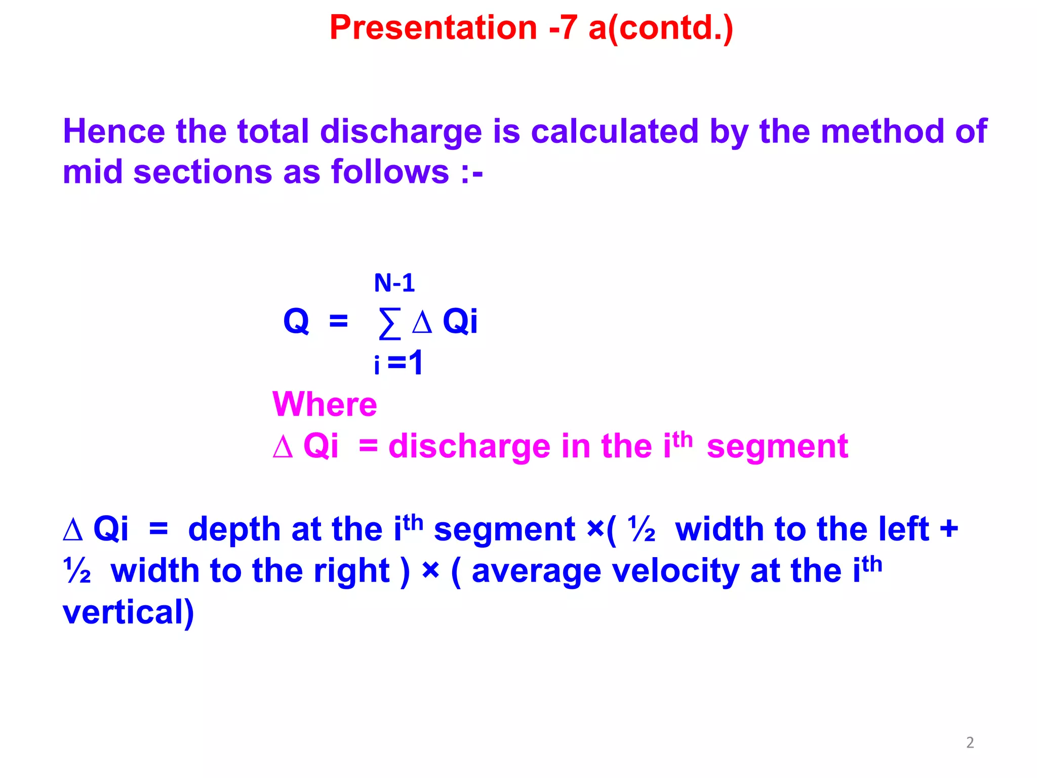
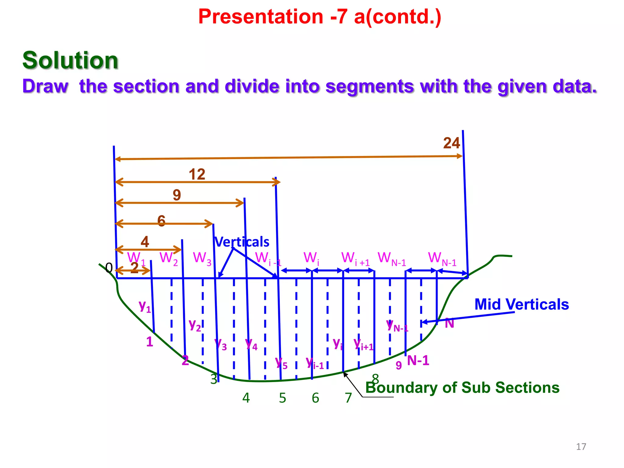
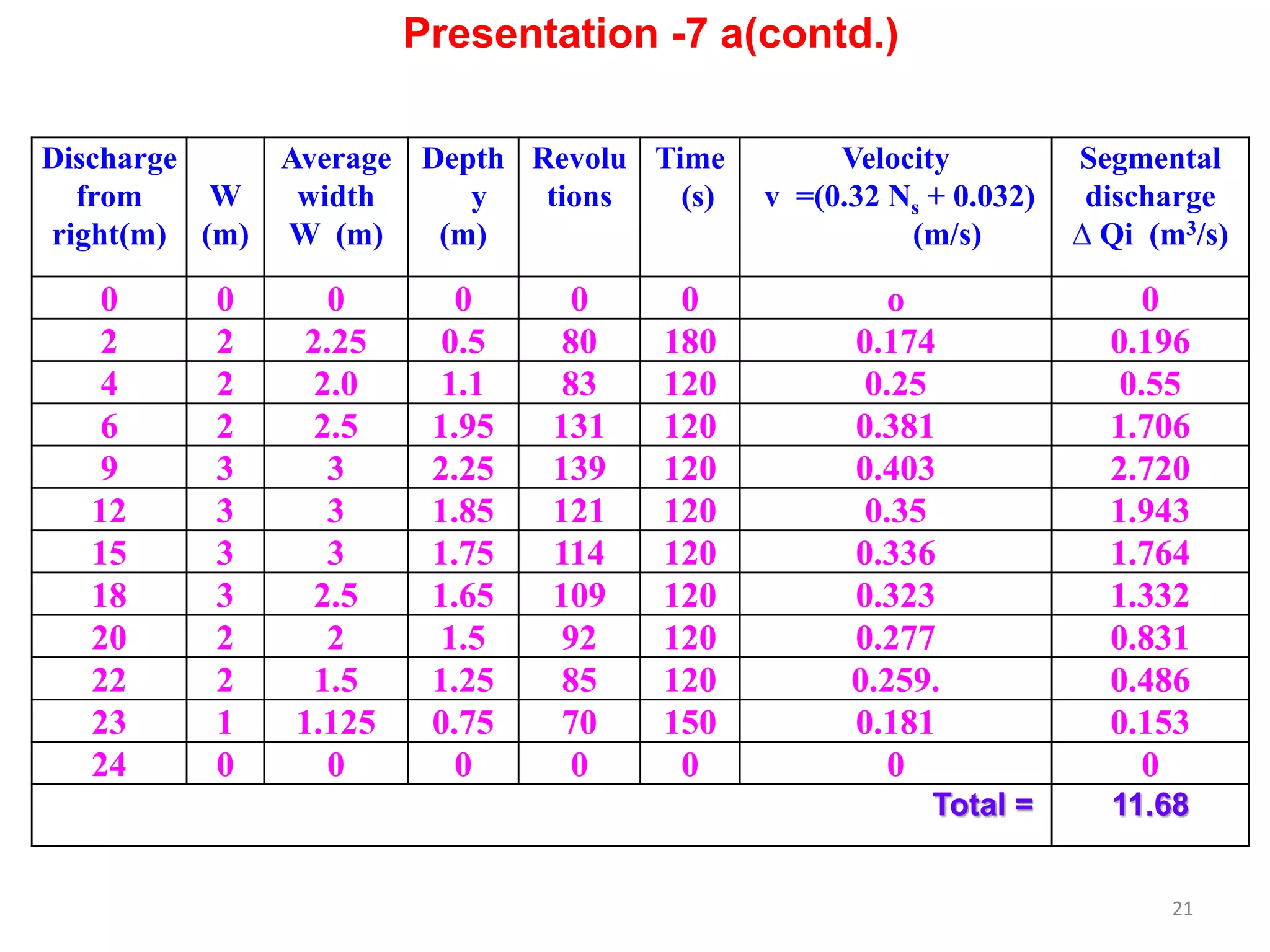
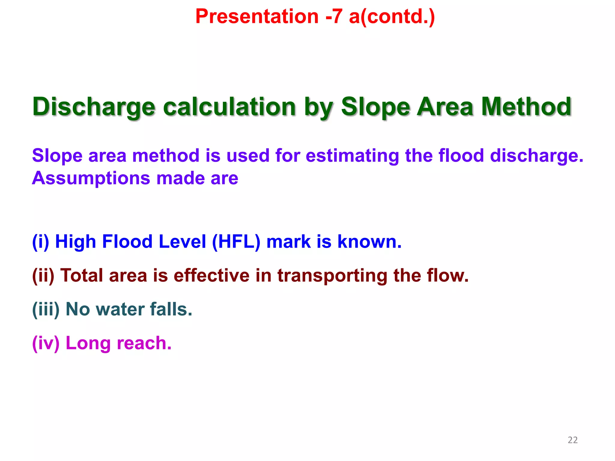
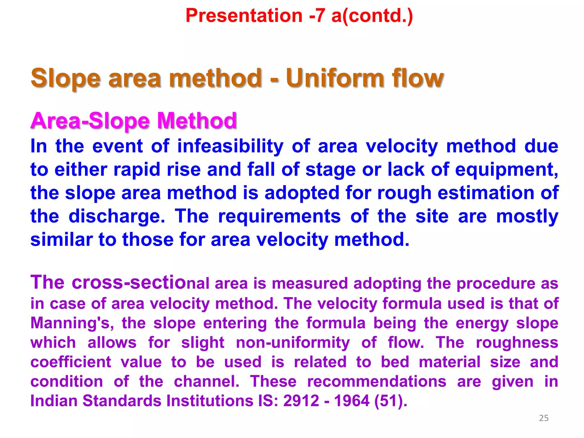
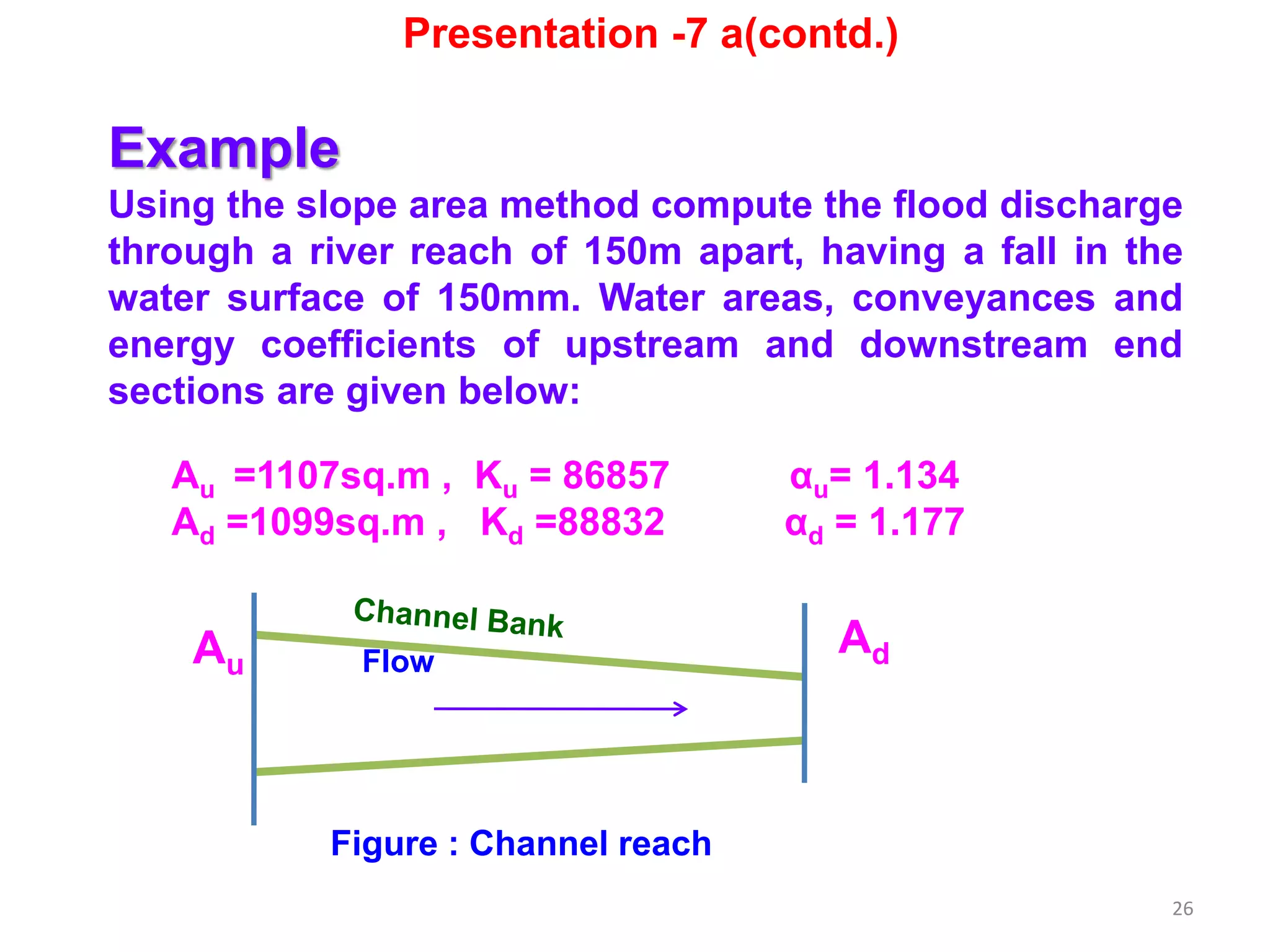
The document describes methods for calculating river discharge, including the area-velocity method and slope-area method. The area-velocity method divides the river cross section into segments, calculates the average width and velocity for each, and sums the segmental discharges. The slope-area method estimates discharge over a long reach based on the high flood level, total flow area, slope of the water surface, and whether the reach is contracting or expanding.

1. 1
Discharge Calculations(Area-Velocity Method)
The Figure below shows the river section where N-1
verticals are drawn. The velocity averaged over the
vertical at each section is known. The total area of the
section is divided into N-1 segments.
Presentation -7 a
W1 W2 W3 W4 W5 W6 WN-1 WN
Fig. River cross section showing segments

2. 2
Hence the total discharge is calculated by the method of
mid sections as follows :-
N-1
Q = ∑ ∆ Qi
i =1
Where
∆ Qi = discharge in the ith segment
∆ Qi = depth at the ith segment ×( ½ width to the left +
½ width to the right ) × ( average velocity at the ith
vertical)
Presentation -7 a(contd.)

3. 3
Discharge at the intermediate section:
∆ Qi = yi × { ( Wi /2) + ( Wi + 1 )/2 } ×vi
Where, i = 2 to N- 2
Average Width and Discharge
(1)Edge Section (average width) :
Left Edge, Wi = {Wi + Wi + 1 /2)} 2 /2Wi
Where, i = 1,2,3,............N
Presentation -7 a(contd.)

4. 4
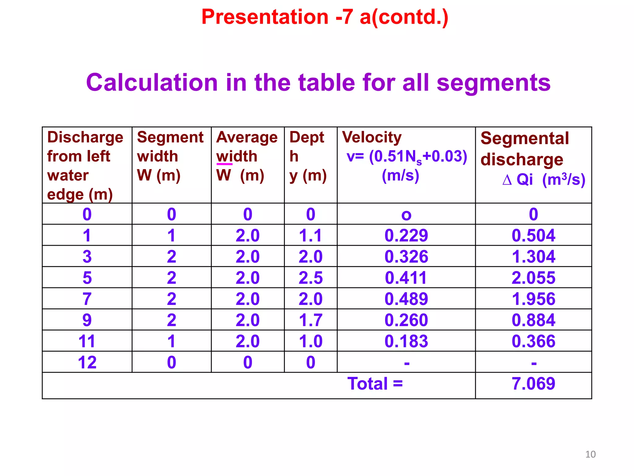
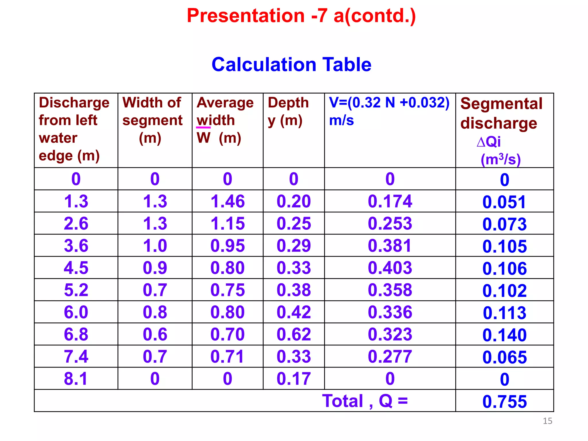
Discharge
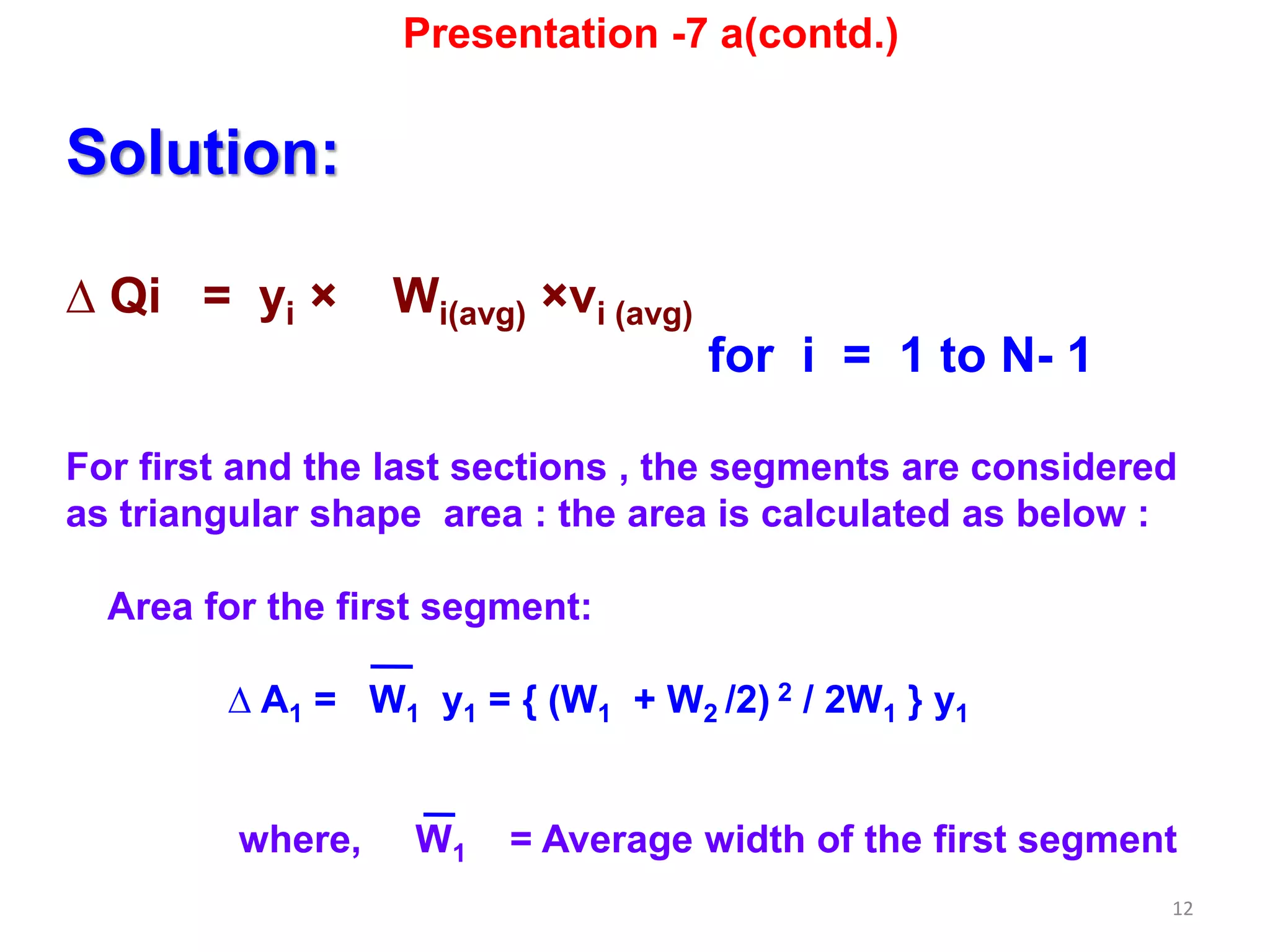
∆ Qi = [{Wi + Wi + 1 /2)} 2 /2Wi]yi vi
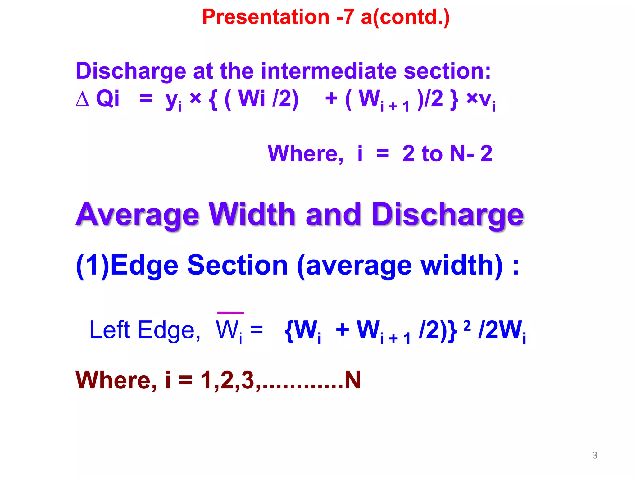
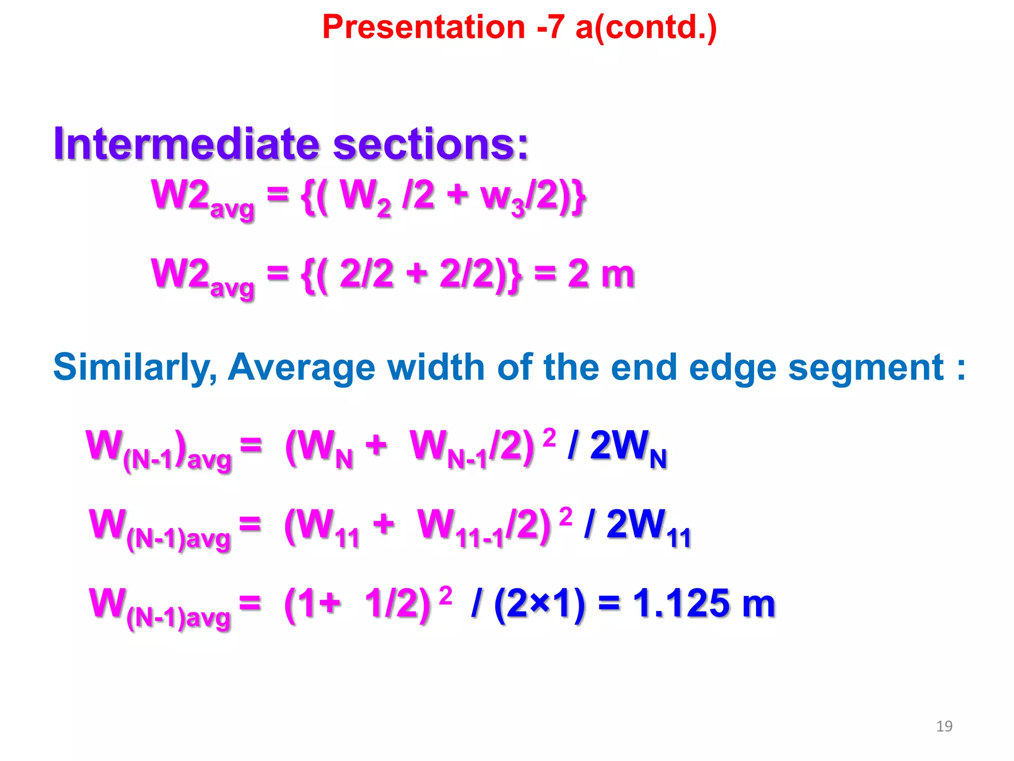
(2) Intermediate Section : average width
Wi = { ( Wi /2) + ( Wi + 1 )/2}
Presentation -7 a(contd.)
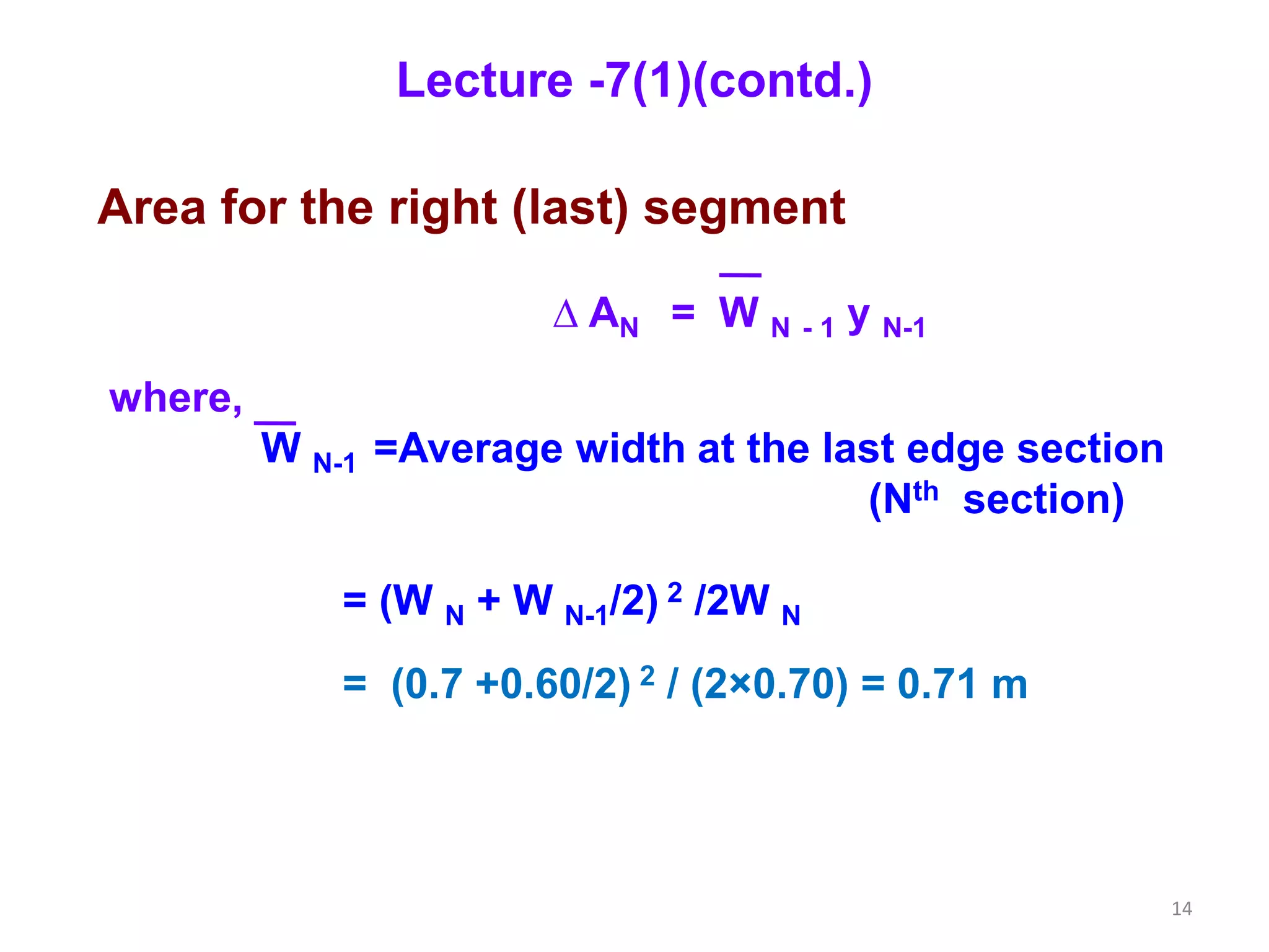
(3) Discharge calculation for Right edge
Average width for right edge
Right Edge, WN-1 = {WN + (WN - 1 /2)} 2 /2WN
∆ Qi = [{WN + WN- 1 /2)} 2 /2WN]yi vi
∆ Qi = (WN- 1)yN-1 vN-1

5. 5
Example 5-2
The data pertaining to a stream-gauging operation at a
gauging site are given in the Table. Calculate the
discharge in the stream. The rating equation for the
current meter (Velocity) is v = (0.51 Ns + 0.03) m/s
Where Ns = Revolution / time
Distance from right
bank(m)
0 1.0 3.0 5.0 7.0 9.0 11.0 12.0
Depth(m) 0 1.1 2.0 2.5 2.0 1.7 1.0 0
Number of revolutions 0 39 58 112 90 45 30 0
Time(s) 0 100 100 150 100 100 100 0
Presentation -7 a(contd.)

6. 6
W1 W2 W3 W4 W5 W6 W7
Mid Verticals/depth
Channel Bed
1.1 2.0 2.5 2.0 1.7 1.0
1.0 m
3.0 m
5.0 m
7.0 m
9.0 m
11.0 m
12.0 m0.0
0.0
Solution
Given , Velocity = v = (0.51 Ns + 0.03) m/s
Other Data in the given table.
Figure :Cross Section
Presentation -7 a(contd.)

7. 7
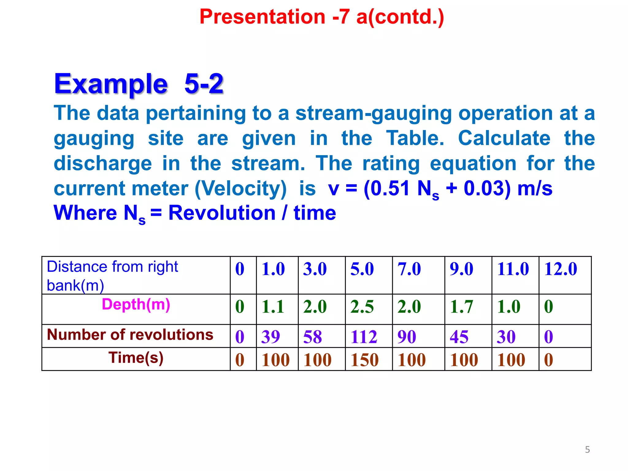
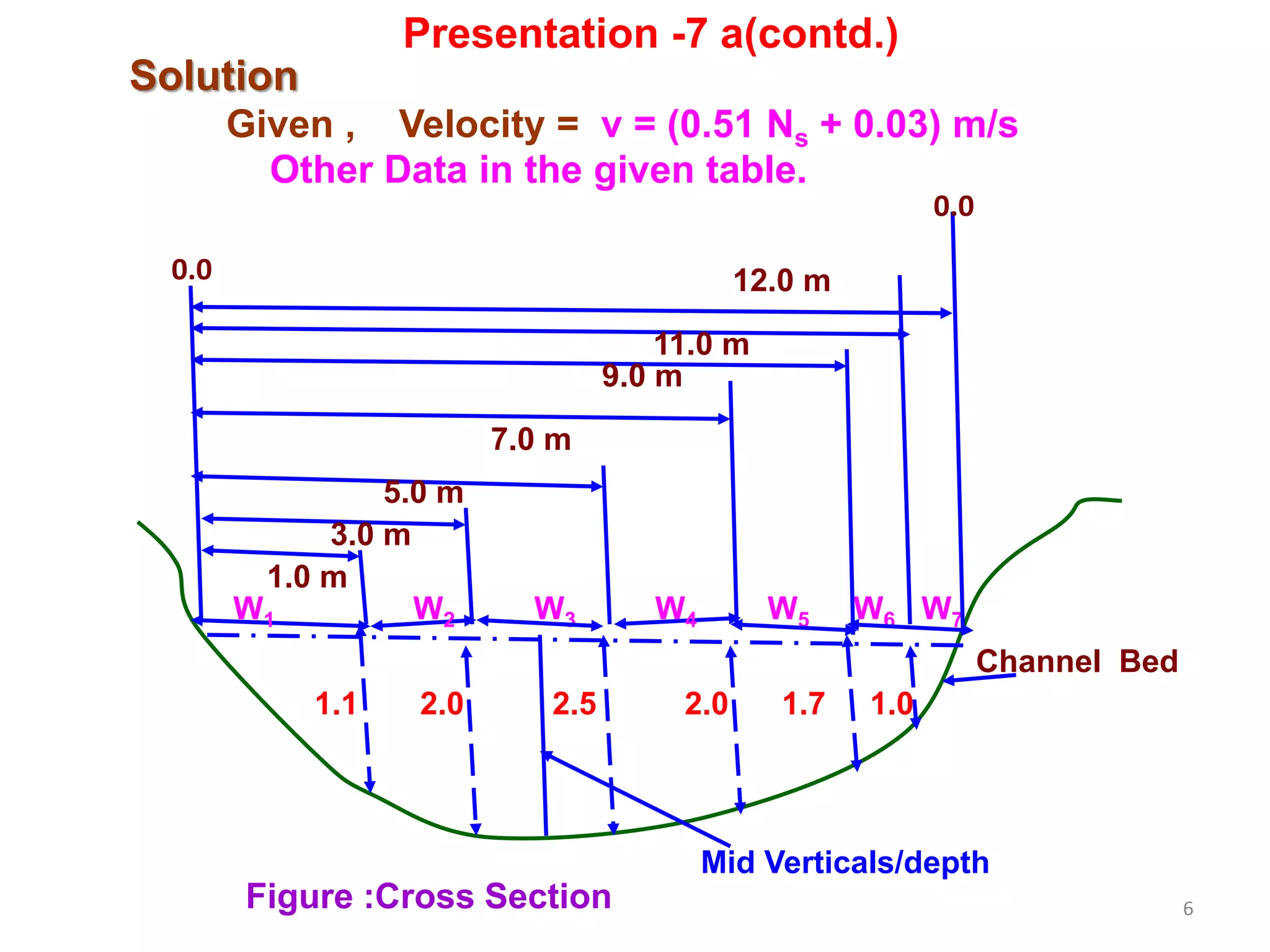
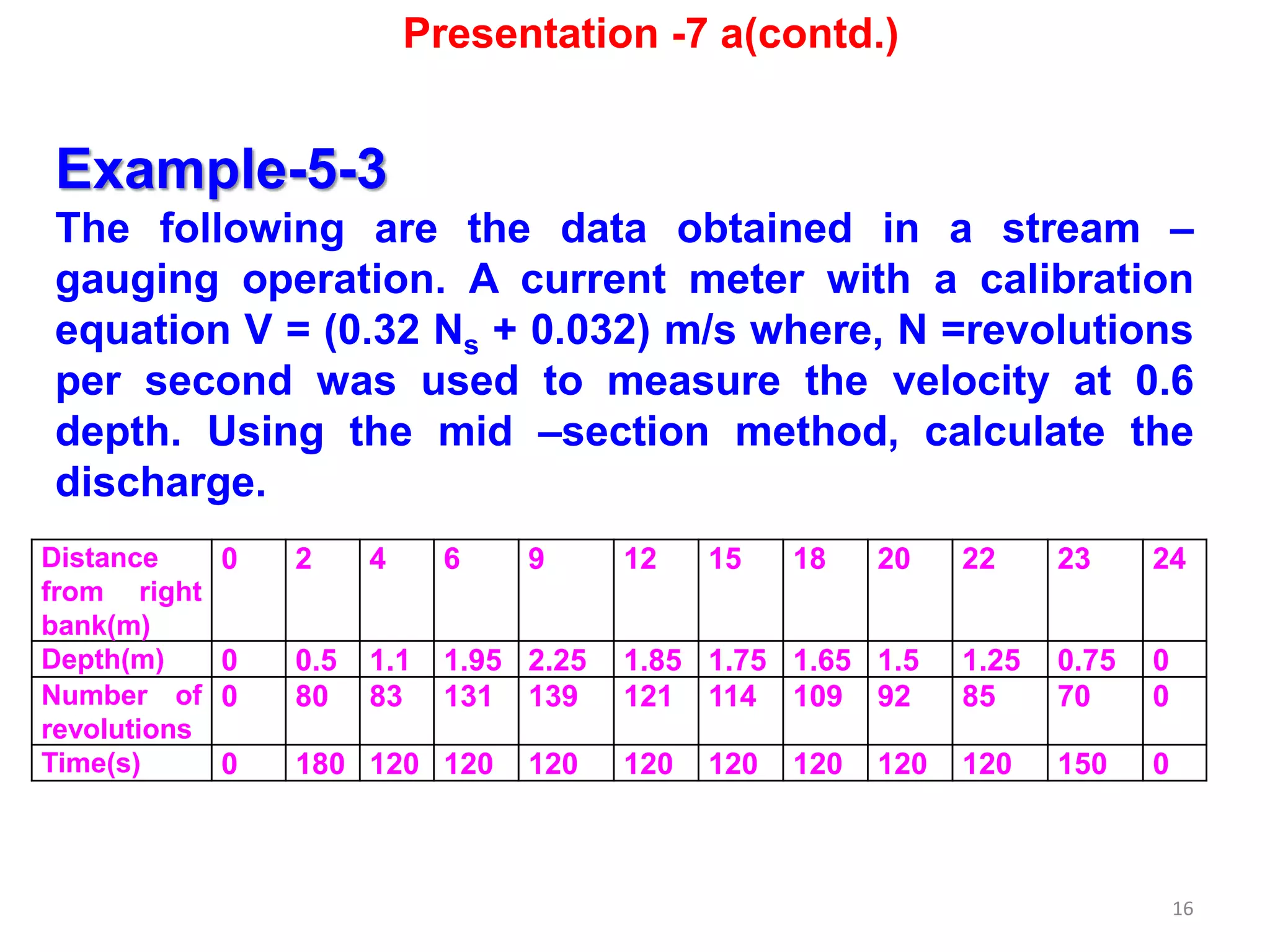
Solution
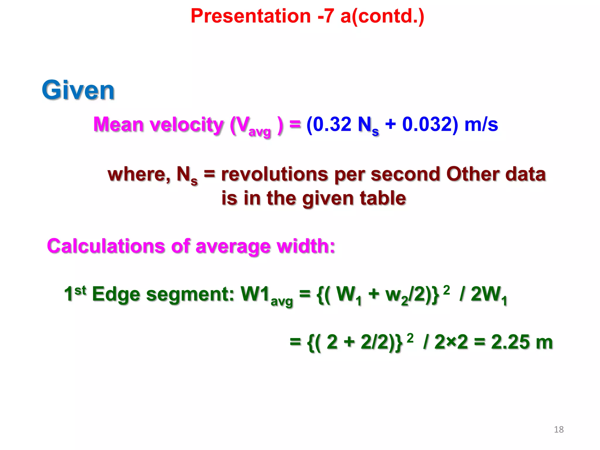
Given,
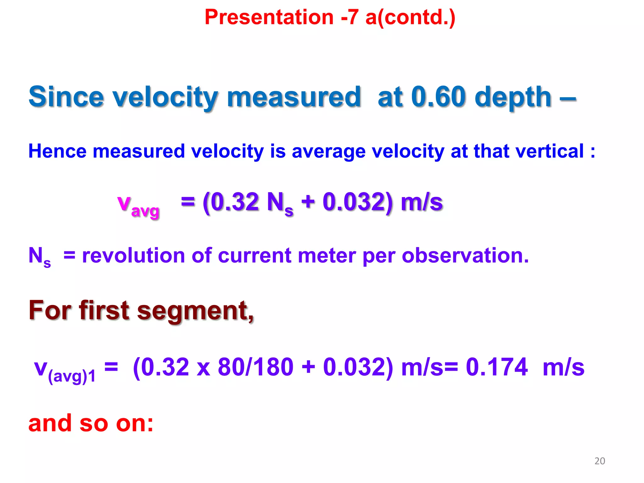
Velocity (v) = (0.51 Ns + 0.03) m/s
where, Ns = Revolution per second
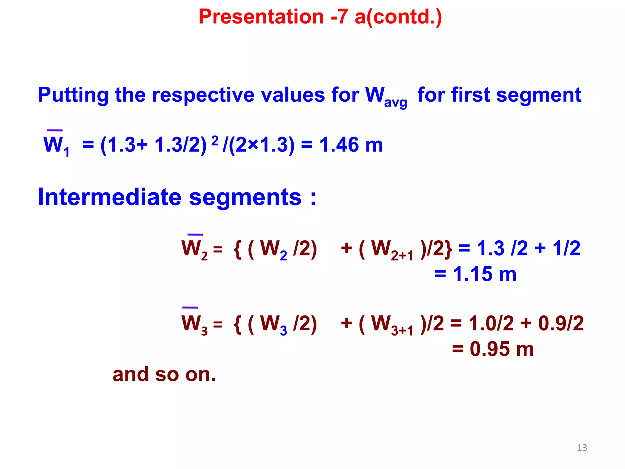
(1) Edge Section (average width = Wavg)
W(avg) = {Wi + Wi + 1 /2)} 2 /2Wi
Left edge discharge
∆ Qi = [{Wi + (Wi + 1 /2)} 2 /2Wi ]× yi × vi(avg)
Wi = Width of ith segment
Where, i = 1,2,3.. N
Presentation -7 a(contd.)

8. 8
W1 = 1.0 m, W2 = 2.0 m, given and so on
Similarly, y1 = 1.10 m, y2 = 2.0 m, and so on given
Putting the values in the above equation for discharge
At the left edge,
∆ Qi = [{1 + 2/2)} 2 /2 ×1] × vi ×yi
v1 = (0.51 × Ns + 0.03) m/s - given
N1 = 39/100 = 0.39
v1 = (0.51 × 0.39 + 0.03) m/s
= 0.229 m/s
Presentation -7 a(contd.)

9. 9
Hence, Discharge at the left edge
Q1 = [{1 + 2/2)} 2 /2 ×1] × 0.229×1.1 = 0.504 m3/s
Discharge for the right edge:
Average width :
Right Edge, WN-1 = {WN + (WN - 1 /2)} 2 /2WN
= {1 + (2 /2)} 2 /2×1 = 2.0 m
Q6 = [{1 + 2/2)} 2 /2 ×1] × 1.0 × 0.183= 0.366 m3/s
Discharge calculation for Intermediate Section
Wi = { ( Wi /2) + ( Wi + 1 )/2}
W2 = { ( W2 /2) + ( W2 + 1 )/2} = 2 m , Q2 = 2× 2.0 ×0.326
=1.304 m3/s
Presentation -7 a(contd.)

10. 10
Discharge
from left
water
edge (m)
Segment
width
W (m)
Average
width
W (m)
Dept
h
y (m)
Velocity
v= (0.51Ns+0.03)
(m/s)
Segmental
discharge
∆ Qi (m3/s)
0 0 0 0 o 0
1 1 2.0 1.1 0.229 0.504
3 2 2.0 2.0 0.326 1.304
5 2 2.0 2.5 0.411 2.055
7 2 2.0 2.0 0.489 1.956
9 2 2.0 1.7 0.260 0.884
11 1 2.0 1.0 0.183 0.366
12 0 0 0 - -
Total = 7.069
Calculation in the table for all segments
Presentation -7 a(contd.)

11. 11
Example-5-3
The following are the data obtained in a stream –gauging
operation. A current meter with a calibration equation
V = (0.32 N + 0.032) m/s where, N =revolutions per second
was used to measure the velocity at 0.6 depth. Using the
mid –section method, calculate the discharge.
Distance
from right
bank(m)
0 1.3 2.6 3.6 4.5 5.2 6.0 6.8 7.4 8.1
Depth(m) 0 0.20 0.25 0.29 0.33 0.38 0.42 0.62 0.33 0.17
Number of
revolutions
0 80 83 131 139 121 114 109 92 85
Time(s) 0 180 120 120 120 120 120 120 120 120
Data Table
Presentation -7 a(contd.)

12. 12
Solution:
∆ Qi = yi × Wi(avg) ×vi (avg)
for i = 1 to N- 1
For first and the last sections , the segments are considered
as triangular shape area : the area is calculated as below :
Area for the first segment:
∆ A1 = W1 y1 = { (W1 + W2 /2) 2 / 2W1 } y1
where, W1 = Average width of the first segment
Presentation -7 a(contd.)

13. 13
Putting the respective values for Wavg for first segment
W1 = (1.3+ 1.3/2) 2 /(2×1.3) = 1.46 m
Intermediate segments :
W2 = { ( W2 /2) + ( W2+1 )/2} = 1.3 /2 + 1/2
= 1.15 m
W3 = { ( W3 /2) + ( W3+1 )/2 = 1.0/2 + 0.9/2
= 0.95 m
and so on.
Presentation -7 a(contd.)

14. 14
Area for the right (last) segment
∆ AN = W N - 1 y N-1
where,
W N-1 =Average width at the last edge section
(Nth section)
= (W N + W N-1/2) 2 /2W N
= (0.7 +0.60/2) 2 / (2×0.70) = 0.71 m
Lecture -7(1)(contd.)

15. 15
Discharge
from left
water
edge (m)
Width of
segment
(m)
Average
width
W (m)
Depth
y (m)
V=(0.32 N +0.032)
m/s
Segmental
discharge
∆Qi
(m3/s)
0 0 0 0 0 0
1.3 1.3 1.46 0.20 0.174 0.051
2.6 1.3 1.15 0.25 0.253 0.073
3.6 1.0 0.95 0.29 0.381 0.105
4.5 0.9 0.80 0.33 0.403 0.106
5.2 0.7 0.75 0.38 0.358 0.102
6.0 0.8 0.80 0.42 0.336 0.113
6.8 0.6 0.70 0.62 0.323 0.140
7.4 0.7 0.71 0.33 0.277 0.065
8.1 0 0 0.17 0 0
Total , Q = 0.755
Calculation Table
Presentation -7 a(contd.)

16. 16
Example-5-3
The following are the data obtained in a stream –
gauging operation. A current meter with a calibration
equation V = (0.32 Ns + 0.032) m/s where, N =revolutions
per second was used to measure the velocity at 0.6
depth. Using the mid –section method, calculate the
discharge.
Distance
from right
bank(m)
0 2 4 6 9 12 15 18 20 22 23 24
Depth(m) 0 0.5 1.1 1.95 2.25 1.85 1.75 1.65 1.5 1.25 0.75 0
Number of
revolutions
0 80 83 131 139 121 114 109 92 85 70 0
Time(s) 0 180 120 120 120 120 120 120 120 120 150 0
Presentation -7 a(contd.)

17. 17
W1 W2 W3 Wi -1 Wi Wi +1 WN-1 WN-1
Verticals
Boundary of Sub Sections
y1
y2 yN-1 N
1 y3 y4 yi yi+1
2 y5 yi-1 9 N-1
3 8
4 5 6 7
Mid Verticals
2
4
6
24
Presentation -7 a(contd.)
Solution
Draw the section and divide into segments with the given data.
0
9
12

18. 18
Given
Mean velocity (Vavg ) = (0.32 Ns + 0.032) m/s
where, Ns = revolutions per second Other data
is in the given table
Calculations of average width:
1st Edge segment: W1avg = {( W1 + w2/2)} 2 / 2W1
= {( 2 + 2/2)} 2 / 2×2 = 2.25 m
Presentation -7 a(contd.)

19. 19
Intermediate sections:
W2avg = {( W2 /2 + w3/2)}
W2avg = {( 2/2 + 2/2)} = 2 m
Similarly, Average width of the end edge segment :
W(N-1)avg = (WN + WN-1/2) 2 / 2WN
W(N-1)avg = (W11 + W11-1/2) 2 / 2W11
W(N-1)avg = (1+ 1/2) 2 / (2×1) = 1.125 m
Presentation -7 a(contd.)

20. 20
Since velocity measured at 0.60 depth –
Hence measured velocity is average velocity at that vertical :
vavg = (0.32 Ns + 0.032) m/s
Ns = revolution of current meter per observation.
For first segment,
v(avg)1 = (0.32 x 80/180 + 0.032) m/s= 0.174 m/s
and so on:
Presentation -7 a(contd.)

21. 21
Discharge
from
right(m)
W
(m)
Average
width
W (m)
Depth
y
(m)
Revolu
tions
Time
(s)
Velocity
v =(0.32 Ns + 0.032)
(m/s)
Segmental
discharge
∆ Qi (m3/s)
0 0 0 0 0 0 o 0
2 2 2.25 0.5 80 180 0.174 0.196
4 2 2.0 1.1 83 120 0.25 0.55
6 2 2.5 1.95 131 120 0.381 1.706
9 3 3 2.25 139 120 0.403 2.720
12 3 3 1.85 121 120 0.35 1.943
15 3 3 1.75 114 120 0.336 1.764
18 3 2.5 1.65 109 120 0.323 1.332
20 2 2 1.5 92 120 0.277 0.831
22 2 1.5 1.25 85 120 0.259. 0.486
23 1 1.125 0.75 70 150 0.181 0.153
24 0 0 0 0 0 0 0
Total = 11.68
Presentation -7 a(contd.)

22. 22
Discharge calculation by Slope Area Method
Slope area method is used for estimating the flood discharge.
Assumptions made are
(i) High Flood Level (HFL) mark is known.
(ii) Total area is effective in transporting the flow.
(iii) No water falls.
(iv) Long reach.
Presentation -7 a(contd.)

23. 23
Also the slope-area approach is justified if the change in
conveyance in the reach is less than 30 percent. Although a
straight, uniform reach is preferred, a contracting reach
should be chosen over an expanding reach if there is a
choice. One or more of the following criteria should be met
in determining the reach length:
(a) The length should be greater than or equal to 75
times the mean depth of flow,
Presentation -7 a(contd.)

24. 24
(b) The fall of the water surface should be equal to or
greater than the velocity head, (If velocity = 1 m/s, V 2 /2g
= 0.05 m and if Velocity 2 m/s , V 2 /2g = 0.20 m) and,
(c) The fall should be equal to or greater than 0.15 m. When
the reach is contracting (Vu < Vd) k = 1.0 When the reach
is expanding (Vu > Vd) , k=0.5. The 50% decrease in the
value of k for an expanding reach is customarily
assumed for the recovery of the velocity head due to the
expansion of the flow.
Presentation -7 a(contd.)

25. 25
Slope area method - Uniform flow
Area-Slope Method
In the event of infeasibility of area velocity method due
to either rapid rise and fall of stage or lack of equipment,
the slope area method is adopted for rough estimation of
the discharge. The requirements of the site are mostly
similar to those for area velocity method.
The cross-sectional area is measured adopting the procedure as
in case of area velocity method. The velocity formula used is that of
Manning's, the slope entering the formula being the energy slope
which allows for slight non-uniformity of flow. The roughness
coefficient value to be used is related to bed material size and
condition of the channel. These recommendations are given in
Indian Standards Institutions IS: 2912 - 1964 (51).
Presentation -7 a(contd.)

26. 26
Example
Using the slope area method compute the flood discharge
through a river reach of 150m apart, having a fall in the
water surface of 150mm. Water areas, conveyances and
energy coefficients of upstream and downstream end
sections are given below:
Au =1107sq.m , Ku = 86857 αu= 1.134
Ad =1099sq.m , Kd =88832 αd = 1.177
Au
AdFlow
Figure : Channel reach
Presentation -7 a(contd.)

27. 27
Solution:
Justification of using Slope -area method
i) {(Kd – ku)/kd} ×100 = {(88832-86857)/88832} ×100
=2.2270 % which is less than 30% hence, slope area
method can be applied.
(ii) Average value of conveyance,
Kavg = √ (Ku Kd) = √ (86857×88832) = 87839
(ii) Assuming initially zero velocity head, energy slope,
Sf = (Fall in water surface in the reach, F )/
(Length of the channel reach, L)
= 0.15/150 = 0.001
Presentation -7 a(contd.)

28. 28
Using Manning’s Formula, Corresponding discharge,
Q1 = Kavg √ Sf = 87839 √ 0.001 = 2777.713 m3/s
For second iteration taking discharge
Q = 2777.713 m3/s
Velocity heads at the upstream and downstream section
respectively-
Velocity upstream, Vu = Q / Au = 2777.713/1107
= 2.5089 m/s
Presentation -7 a(contd.)

29. 29
Velocity down stream = Q/Ad = 2777.713/1099
= 2.25270 m/s
As we know, if Vu < Vd
then, K = 1.0 and
if Vu > Vd
then , K = 0.5
(i) Velocity head (upstream),
α uVu
2 /2g = α u (Q/Au) 2 /2g
= 1.134×2777.713/ 1107) 2 /2×9.81
= 0.364 m
Presentation -7 a(contd.)

30. 30
(ii) Velocity head (down stream)
α dVd
2 /2g = αd (Q/Ad) 2/2g
= 1.177 (2777.713/1099) 2/2×9.81
= 0.383 m
The difference in the velocity head is equal to
0.364 -0.383 = -0.019 m
Frictional Head loss, hf = 0.15 – 0.019 = 0.131 m
For third iteration taking discharge :
Revised energy slope , Sf = 0.131/ 150
= 0.000873
Presentation -7 a(contd.)

31. 31
Revised Discharge , Q2 = Kavg √ Sf = 87839 √ 0.000873
= 2596 m3/s
(i) Velocity head (upstream),
α uVu
2 /2g = α u (Q/Au) 2 /2g
= 1.134×2596/ 1107) 2 /2×9.81
= 0.318 m
(ii) Velocity head (down stream)
α dVd
2 /2g = αd (Q/Ad) 2/2g = 1.177× 2596/1099)2/2×9.81
= 0.335 m
Presentation -7 a(contd.)

32. 32
The difference in the velocity head is equal to
0.318 -0.335 = -0.017 m
Frictional Head loss, hf = 0.15 – 0.017 = 0.133m
Revised energy slope , Sf = 0.133/ 150 = 0.000866
Revised Discharge , Q3 = Kavg √ Sf
= 87839 √ 0.000866 = 2615 m3/s
And so on
Data Table
Sl.No. ɑu(Vu
2 )/2g
(m)
ɑd(Vd
2 )/2g
(m)
V2/2g
(m)
hf
(m)
Sf Q
(m3/s)
1. - - - 0.15 0.001 2777.713
2. 0.364 0.383 - 0.019 0.131 0.000873 2596
3. 0.318 0.335 -0.017 0.133 0.000866 2615
4. 0.3225 0.34 -0.0175 0.1325 0.000883 2611
Flood discharge through the given river reach Q =2611 m3/s)
Presentation -7 a(contd.)