LABORATORY REPORT : Discharge measurement using a current meter

1. 1
College of Engineering
Civil Engineering Department
Water Resources Engineering – CE341
LABORATORY REPORT
The experiment number: 9
The experiment title: Discharge measurement using a current meter
Date of experiment:
Due date of the report:
Student Name: ID: :
(Fall Session- 2020)
Dr. Sultan Salamah

2. 2
TABLE OF CONTENTS
1.1. OBJECTIVES...........................................................................................................................3
1.2. THEORY ..................................................................................................................................3
1.3. EXPERIMENT APPARATUS AND SETUP..........................................................................4
1.3.2 SETUP (If any)...................................................................................................................4
1.4. EXPERIMENT PROCEDURES AND MATHEMATICAL EQUATIONS...........................5
1.4.1 Relation between Mean Velocity and Mean Surface Velocity...........................................5
1.4.2 Estimation of Surface Velocity with Velocity Distribution Based on Probability.............6
1.4.3 Estimation of Cross Section Area and Discharge...............................................................7
1.5 OBSERVATIONS & CALCULATIONS .................................................................................8
1.6 RESULTS AND DISCUSSIONS..............................................................................................9
References......................................................................................................................................11
TABLE OF Figures
Figure 1 A magnetic-inductive current meter and a SVR are used at the Guanyin Bridge............ 4
Figure2 A down-looking SW integrated with a sounding weight is used to measure the velocity
profiles in the Longen Channel....................................................................................................... 4
Figure3 Mid-section method of computing cross-section area and stream discharge................... 6
Figure4 Velocity field in the η − ξ coordinate system with a set of isovels. (a) h ≤ 0; (b) h > 0. 7
Figure5 Relation between mean velocities of cross section and surface. the Nankang River at the
Guanyin Bridge............................................................................................................................... 8
Figure6 the Longen Channel.......................................................................................................... 9
Figure7 Accuracy of discharge measurement by surface mean velocity; the Longen Channel . 10
Figure8 the Nankang River at the Guanyin Bridge ..................................................................... 10

3. 3
1.1. OBJECTIVES
After completing this Experiment exercise, we should be able to measure the velocity, discharge
and cross-sectional area of small streams
1.2. THEORY
Conventional methods of river discharge measurement apply the velocity-area principle [1] for
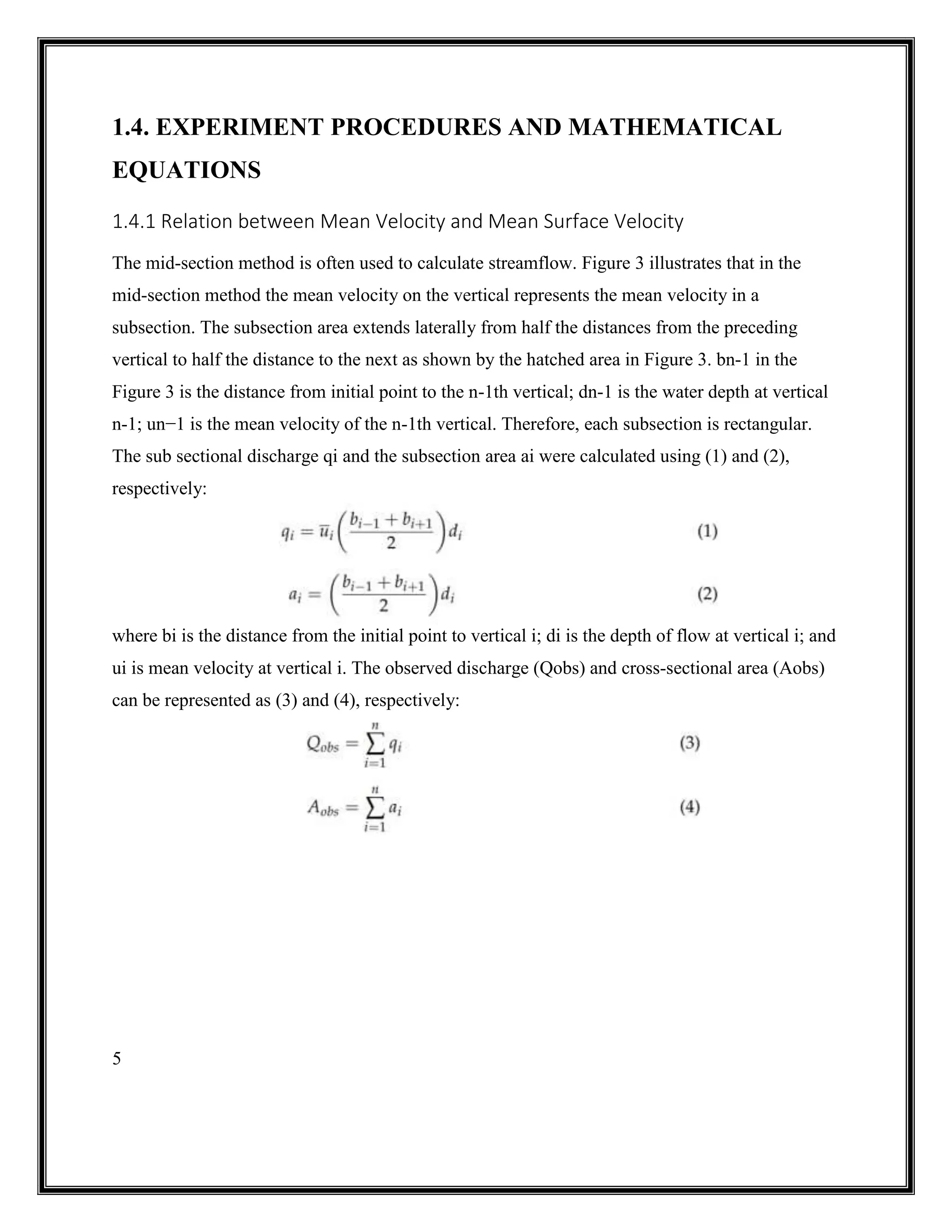
field measurements while the mid-section method [2] is used to calculate the streamflow. The
conventional method involves dividing a river cross-section into several subsections. In each
subsection, the mean velocity and water depth are measured along the vertical to obtain the
discharge of the subsection. The streamflow is the sum of the discharge measurements of all
subsections. The conventional method is usually a contact method, requiring a current meter, a
sounding weight, and hydrologists on site making this method costly, time-consuming, and
labor-intensive. This method is not suitable for tidal streams and during the high water.
Many instruments have been invented with the goal of improving conventional methods,
allowing for the rapid and accurate measurement of flow velocity and water depth.
An acoustic Doppler current profiler (ADCP) which applies the Doppler Effect is a relatively
new instrument and has been widely considered as a method used to replace mechanical current
meters for velocity measurement. Simpson [3] used a broad-band ADCP that is much faster for
accurately measuring tidally affected flow than conventional methods. Boiten [4] applied ADCPs
to measure discharges in open channels, according to the velocity-area principle. Costa et al.
[5,6] used a boat-mounted ADCP to measure discharge for converting surface-velocity to mean
velocity. Muste et al. [7] analyzed velocity profiles collected by ADCPs to propose
complementary software for better support of hydraulic investigation requirements. Chauhan et
al. [8] showed that the relative error of the discharge measurement is very small with the ADCP
compared to the conventional method. Oberg and Mueller [9] showed that ADCP streamflow
measurements are unbiased when compared to the discharges obtained by current meter, stable
rating curves, salt-dilution, and acoustic velocity meter. Flener et al. [10] used the

4. 4
multidimensional spatial flow patterns measured by an ADCP installed on a remotely controlled
boat to monitor a spring flood.
Ground penetration radar [11,12], lidar [13], pressure sensors, and sonar systems [
14,15
] have
been developed to replace the conventional sounding weights during water depth measurement.
Although these modern instruments are costlier, they can be applied to provide data when
conventional instruments cannot, with the extra benefits of reducing the overall cost and time
required [
10,16
.]
1.3. EXPERIMENT APPARATUS AND SETUP
1.3.2 SETUP (If any)
Figure 1 A magnetic-inductive current meter and a SVR are
used at the Guanyin Bridge
Figure 2 A down-looking SW integrated with a sounding weight is used
to measure the velocity profiles in the Longen Channel

5. 5
1.4. EXPERIMENT PROCEDURES AND MATHEMATICAL
EQUATIONS
1.4.1 Relation between Mean Velocity and Mean Surface Velocity
The mid-section method is often used to calculate streamflow. Figure 3 illustrates that in the
mid-section method the mean velocity on the vertical represents the mean velocity in a
subsection. The subsection area extends laterally from half the distances from the preceding
vertical to half the distance to the next as shown by the hatched area in Figure 3. bn-1 in the
Figure 3 is the distance from initial point to the n-1th vertical; dn-1 is the water depth at vertical
n-1; un−1 is the mean velocity of the n-1th vertical. Therefore, each subsection is rectangular.
The sub sectional discharge qi and the subsection area ai were calculated using (1) and (2),
respectively:
where bi is the distance from the initial point to vertical i; di is the depth of flow at vertical i; and
ui is mean velocity at vertical i. The observed discharge (Qobs) and cross-sectional area (Aobs)
can be represented as (3) and (4), respectively:

6. 6
1.4.2 Estimation of Surface Velocity with Velocity Distribution Based on Probability
The surface velocity can be measured directly by SVR in most conditions. However, when the
channel width is not enough for accommodating the instrument, one can measure the velocity
profile on each vertical and use the velocity distribution equation to estimate the surface velocity.
This study applied the probabilistic velocity distribution to estimate the surface velocity [24],
which is shown in (11):
where umax is the max velocity; M is a parameter; ξ is the isovel in Figure 4 [25]; u is the
velocity at ξ; ξmax and ξ0 are the values of ξ at which u = umax and u = 0, respectively. In
addition, a η − ξ coordinate system can be used to describe the velocity field with a set of isovels,
in which ξ and u has a one-to-one relationship, meaning that the velocities are the same on ξ,
unlike the Cartesian coordinate system where the same velocity values can occur in difference
locations. The ξ on the vertical line is shown in (12):
Figure 3 Mid-section method of computing cross-section area and stream discharge

7. 7
1.4.3 Estimation of Cross Section Area and Discharge
In practice, there are many approaches for cross-sectional area estimation under different
conditions. For a fixed artificial channel, the water stage is consistent enough that it can be used
for estimating the cross-sectional area. For a stable channel bed without obvious erosion and
sediment deposition, the relationship between the water stage and the cross-sectional area can be
used to estimate the cross-sectional area of the river. For an unstable channel bed, the cross-
sectional area can be estimated from the water depth of the verticals [26] using (13):
Figure 4 Velocity field in the η − ξ coordinate system with a
set of isovels. (a) h ≤ 0; (b) h > 0.

8. 8
1.5 OBSERVATIONS & CALCULATIONS
When all the points were combined, all the points fall on the periphery of the regression line, and
when the mean surface velocity increases, the data tends to approach the regression line. This
means that as the water depth increases, the width of the crosssection increases even more
making the shape of the cross-section approach the shape of a rectangle. Hence, the relationship
between the mean surface velocity and the mean velocity was stable. Figure 6 shows an artificial
rectangular channel with all the points falling near the regression line. This means that the
relationship between us and Uobs of the artificial rectangular channel is very stable. It reveals
that the mean cross-sectional velocity and mean surface velocity in both the natural and the
artificial channels have correlation coefficients of 0.92 and 0.99, respectively. As the artificial
channel is confined with the concrete bed and walls, the velocity is less affected by natural
factors; and thus, it performs better than the natural channel. Figure 5 demonstrates that the
relationship between the mean surface velocity and the mean velocity of natural rivers and
artificial channels is quite stable, forming a linear relationship through the origin.
Figure 5 Relation between mean velocities of cross section and surface.
the Nankang River at the Guanyin Bridge

9. 9
1.6 RESULTS AND DISCUSSIONS
The discharge measurement in the natural channel at the Guanyin Bridge was taken by the
conventional two-point method for the water depth and the mean vertical velocity. Meanwhile,
owing to the limitations caused by the channel width, the discharge measurement at the Longen
Channel was taken from the vertical velocity profile for the mean velocity. The mid-section
method was then applied to both the natural and the artificial channels. The mean cross-sectional
velocity can be observed by the discharge divided by the cross-sectional area. Figure 7 shows the
vertical velocity profile of the Longen Channel on 8 March 2019 when the discharge was 3.80
m3/s. The flow pattern of the Longen Channel was quite similar to a large-scale hydraulic flume
in a laboratory. In Figure 7, it is obvious that the flow patterns of Longen Channel were very
different from those of natural rivers. Most of the maximum velocities on the verticals occurred
Figure 6 the Longen Channel

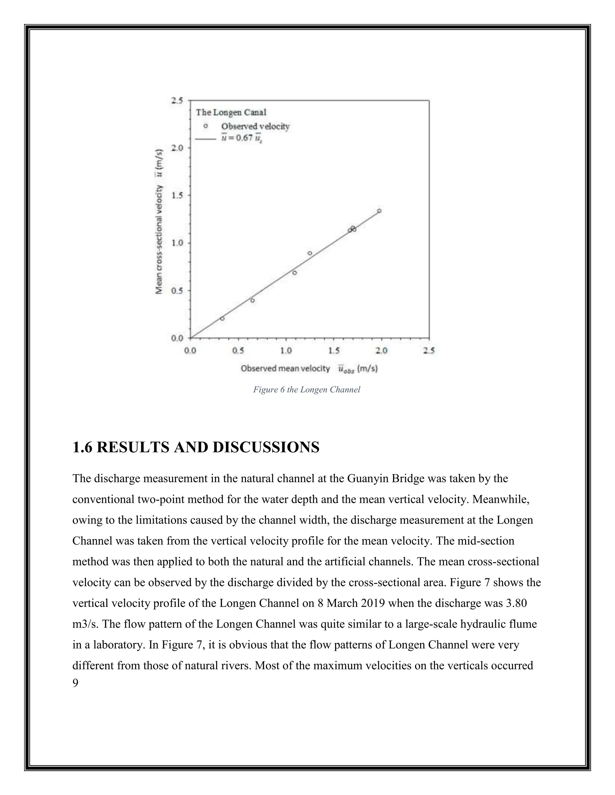
10. 10
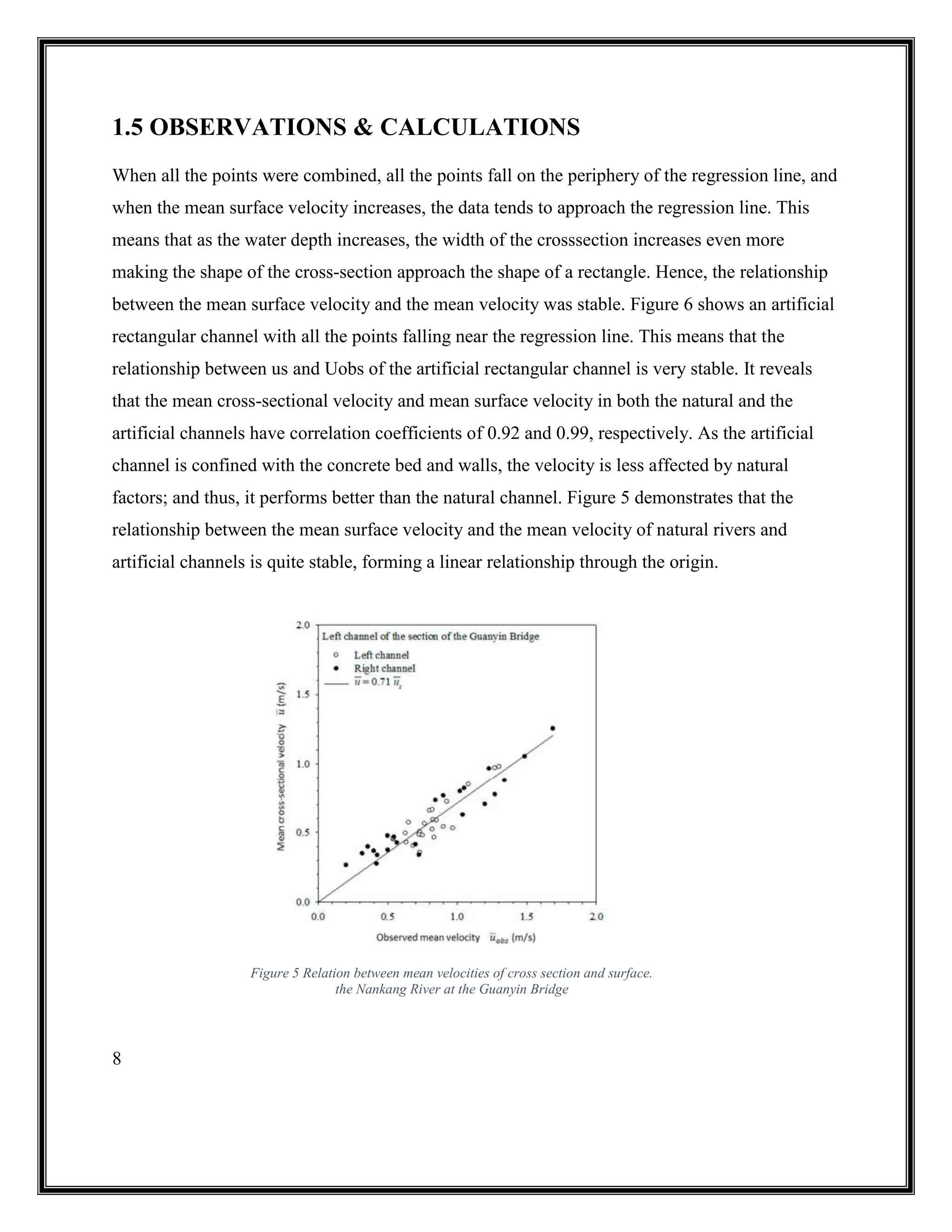
at a depth of about 1/4 water depth from the water surface, while the surface velocity was
relatively small. It also shows that the maximum velocities of the verticals excluding verticals (e)
and (f) did not occur on the water surface. Experimental studies have been shown from
considerations of momentum transfer that the velocity in an open channel should decrease
toward the channel bed. In a very wide channel the velocity decreases toward the bed and walls,
and theoretically the maximum occurs at the water surface. The Longen Channel is a small
artificial flume; therefore, depression of the maximum velocities below the water surface was
observed. The flow pattern cannot be described by a logarithmic distribution. The circle in
Figure 7 is the actual velocity measurement on each vertical, and the line is the velocity
distributions based on (11) indicating that vertical maximum velocity does not always occur on
the water surface. It also shows that the velocity profile data of the Longen Channel is difficult to
describe using conventional velocity distribution theories, such as logarithm velocity
distribution. However, (11) can simulate velocity profiles effectively, regardless of whether the
maximal velocity occurs on or below the water surface. Therefore, the surface velocities on the
verticals could also obtained precisely by using (11). In addition, using the nonlinear regression
method, M, h and umax can also be obtained from (11) with the vertical velocity and water
depth. Thus, the mean vertical velocity (ui in [1]) on each vertical can be estimated. Therefore
(11) can be used to accurately estimating the mean velocity of the vertical for obtaining reliable
discharge.
Figure 8 the Nankang River at the Guanyin Bridge
Figure 7 Accuracy of discharge measurement
by surface mean velocity; the Longen
Channel

11. 11
References
[ 1 ] Herschy, R.W. Streamflow Measurement; Routledge: New York, NY, USA, 2009.
[CrossRef]
[ 2 ] Rantz, S.E. Measurement and Computation of Streamflow: Volume 1. Measurement of
Stage and Discharge; USGS Water Supply Paper 2175; U.S. Government Printing Office:
Washington, DC, USA, 1982. [CrossRef]
[ 3 ] Simpson, M.R. Discharge Measurements Using a Broad-Band Acoustic Doppler Current
Profiler; US Geological Survey: Sacramento,CA, USA, 2001.
[ 4 ] Boiten, W. Hydrometry, 1st ed.; CRC Press: Lisse, The Netherlands, 2003.
[ 5 ] Costa, J.E.; Spicer, K.R.; Cheng, R.T.; Haeni, F.P.; Melcher, N.B.; Thurman, E.M.; Plant,
W.J.; Keller, W.C. Measuring stream discharge by non-contact methods—A proof-of-
concept experiment. Geophys. Res. Lett. 2000, 27, 553–556. [CrossRef]
[ 6 ] Costa, J.E.; Cheng, R.T.; Haeni, F.P.; Melcher, N.; Spicer, K.R.; Hayes, E.; Plant, W.;
Hayes, K.; Teague, C.; Barrick, D. Use of radars to monitor stream discharge by
noncontact methods. Water Resource. Res. 2006, 42, W07422. Available online:
https://agupubs.onlinelibrary.wiley.com/doi/epdf/10.1029/2005WR004430 (accessed on
26 July 2022). [CrossRef]
[ 7 ] Muste, M.; Yu, K.; Spasojevic, M. Practical aspects of ADCP data use for quantification
of mean river flow characteristics; part I: Moving-vessel measurements. Flow Meas.
Instrum. 2004, 15, 1–16. [CrossRef]
[ 8 ] Chauhan, M.S.; Kumar, V.; Dikshit, P.K.S.; Dwivedi, S.B. Comparison of discharge data
using ADCP and current meter. Int. J. Adv. Earth Sci. 2014, 3, 81–86.
[ 9 ] Oberg, K.A.; Mueller, D.S. Validation of streamflow measurements made with acoustic
Doppler current profilers. J. Hydraul. Eng.2007, 133, 1421–1432. [CrossRef]
[ 10 ] Flener, C.; Wang, Y.; Laamanen, L.; Kasvi, E.; Vesakoski, J.M.; Alho, P. Empirical
modeling of spatial 3d flow characteristics using a remote-controlled ADCP system:
Monitoring a spring flood. Water 2015, 7, 217–247. [CrossRef]

12. 12
[ 11 ] Chen, Y.C.; Kao, S.-P.; Wu, C.-H. Measurement of stream cross section using ground
penetration radar with Hilbert–Huang transform. Hydrol. Process. 2014, 28, 2468–2477.
[CrossRef]
[ 12 ] Chen, Y.C.; Kao, S.P.; Hsu, Y.C.; Chang, C.W.; Hsu, H.-C. Automatic measurement and
computation of stream cross-sectional area using ground penetrating radar with an
adaptive filter and empirical mode decomposition. J. Hydrol. 2021, 600, 126665.
[CrossRef]
[ 13 ] Mitchell, S.; Thayer, J.P.; Hayman, M. Polarization lidar for shallow water depth
measurement. Appl. Opt. 2010, 49, 6995–7000.[CrossRef]
[ 14 ] Gupta, S.D.; Shahinur, I.M.; Haque, A.A.; Ruhul, A.; Majumder, S. Design and
implementation of water depth measurement and object detection model using ultrasonic
signal system. Int. J. Eng. Res. Dev. 2012, 4, 62–69.
[ 15 ] Chen, Y.-C.; Yang, C.-M.; Hsu, N.-S.; Kao, T.-M. Real-time discharge measurement in
tidal streams by an index velocity. Environ. Monit. Assess. 2012, 184, 6423–6436.
[CrossRef]
[ 16 ] U.S. Geological Survey (USGS). Streamflow Information for the Next Century—A Plan
for the National Streamflow Information Program of the U.S. Geological Survey; USGS
Open-File Report 99-456; U.S. Geological Survey: Reston, VA, USA, 1999. [CrossRef]
[ 17 ] Gença, O.; Ardıçlıo ˘glu, M.; A ˘gıralio ˘glu, N. Calculation of mean velocity and
discharge using water surface velocity in small streams. Flow Meas. Instrum. 2014, 41,
115–120. [CrossRef]
[ 18 ] Chen, Y.C.; Liao, Y.J.; Chen, W.-L. Discharge estimation in lined irrigation channels by
using surface velocity radar. Paddy Water Environ. 2018, 16, 857–866. [CrossRef]
[ 19 ] Novak, G.; Rak, G.; Prešerena, T.; Bajcar, T. Non-intrusive measurements of shallow
water discharge. Flow Meas. Instrum. 2017, 56, 14–17. [CrossRef]
[ 20 ] Welber, M.; Coz, J.L.; Laronne, J.B.; Zolezzi1, G.; Zamler, D.; Dramais, G.; Hauet, A.;
Salvaro, M. Field assessment of noncontact stream gauging using portable surface
velocity radars (SVR). Water Resour. Res. 2016, 52, 1108–1126. [CrossRef]

13. 13
[ 21 ] Legleiter, C.J.; Kinzel, P.J.; Nelson, J.M. Remote measurement of river discharge using
thermal particle image velocimetry (PIV) and various sources of bathymetric
information. J. Hydrol. 2017, 554, 490–506. [CrossRef]
[ 22 ] Hauet, A.; Morlot, T.; Daubagnan, L. Velocity profile and depth-averaged to surface
velocity in natural streams: A review over a large sample of rivers. E3S Web Conf. 2018,
40, 06015. [CrossRef]
[ 23 ] Corato, G.; Ammari, A.; Moramarco, T. Conventional point-velocity records and surface
velocity observations for estimating high flow discharge. Entropy 2014, 16, 5546–5559.
[CrossRef]
[ 24 ] Chiu, C.L. Velocity distribution in open-channel flow. J. Hydraul. Eng. 1989, 115, 576–
594. [CrossRef]
[ 25 ] Chiu, C.L. Entropy and 2-D velocity distribution in open-channels. J. Hydraul. Eng.
1988, 114, 738–756. [CrossRef]
[ 26 ] Chen, Y.C.; Chiu, C.L. A fast method of flood discharge estimation. Hydrol Process.
2004, 18, 1671–1684. [CrossRef]