Today’s discussion…
Statisticsversus Probability
Concept of random variable
Probability distribution concept
Discrete probability distribution
Continuous probability distribution
Concept of sampling distribution
Major sampling distributions
Usage of sampling distributions
2
3.
3
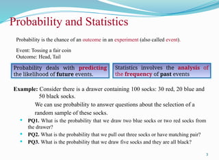
Probability deals withpredicting
the likelihood of future events.
Example: Consider there is a drawer containing 100 socks: 30 red, 20 blue and
50 black socks.
We can use probability to answer questions about the selection of a
random sample of these socks.
PQ1. What is the probability that we draw two blue socks or two red socks from
the drawer?
PQ2. What is the probability that we pull out three socks or have matching pair?
PQ3. What is the probability that we draw five socks and they are all black?
Statistics involves the analysis of
the frequency of past events
Probability is the chance of an outcome in an experiment (also called event).
Event: Tossing a fair coin
Outcome: Head, Tail
Probability and Statistics
4.
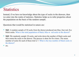
Instead, if wehave no knowledge about the type of socks in the drawers, then
we enter into the realm of statistics. Statistics helps us to infer properties about
the population on the basis of the random sample.
Questions that would be statistical in nature are:
SQ1: A random sample of 10 socks from the drawer produced one blue, four red, five
black socks. What is the total population of black, blue or red socks in the drawer?
SQ2: We randomly sample 10 socks, and write down the number of black socks and
then return the socks to the drawer. The process is done for five times. The mean
number of socks for each of these trial is 7. What is the true number of black socks in
the drawer?
etc.
4
Statistics
5.
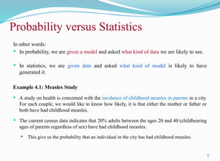
In other words:
In probability, we are given a model and asked what kind of data we are likely to see.
In statistics, we are given data and asked what kind of model is likely to have
generated it.
Example 4.1: Measles Study
A study on health is concerned with the incidence of childhood measles in parents in a city.
For each couple, we would like to know how likely, it is that either the mother or father or
both have had childhood measles.
The current census data indicates that 20% adults between the ages 20 and 40 (childbearing
ages of parents regardless of sex) have had childhood measles.
This give us the probability that an individual in the city has had childhood measles.
5
Probability versus Statistics
6.
Defining Random Variable
6
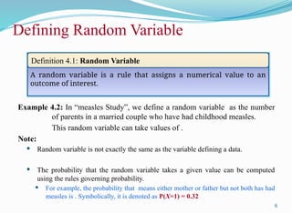
Arandom variable is a rule that assigns a numerical value to an
outcome of interest.
Definition 4.1: Random Variable
Example 4.2: In “measles Study”, we define a random variable as the number
of parents in a married couple who have had childhood measles.
This random variable can take values of .
Note:
Random variable is not exactly the same as the variable defining a data.
The probability that the random variable takes a given value can be computed
using the rules governing probability.
For example, the probability that means either mother or father but not both has had
measles is . Symbolically, it is denoted as P(X=1) = 0.32
7.
Probability Distribution
7
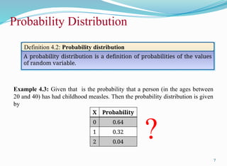
A probabilitydistribution is a definition of probabilities of the values
of random variable.
Definition 4.2: Probability distribution
Example 4.3: Given that is the probability that a person (in the ages between
20 and 40) has had childhood measles. Then the probability distribution is given
by
X Probability
0 0.64
1 0.32
2 0.04
?
8.
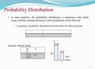
In dataanalytics, the probability distribution is important with which
many statistics making inferences about population can be derived .
In general, a probability distribution function takes the following form
Example: Measles Study
8
0 1
2
0.64 0.32
0.04
Probability Distribution
0.64
0.32
0.04
x
f(x)
9.
9
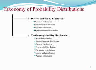
Discrete probability distributions
Binomialdistribution
Multinomial distribution
Poisson distribution
Hypergeometric distribution
Continuous probability distributions
Normal distribution
Standard normal distribution
Gamma distribution
Exponential distribution
Chi square distribution
Lognormal distribution
Weibull distribution
Taxonomy of Probability Distributions
10.
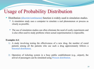
Usage of ProbabilityDistribution
10
Distribution (discrete/continuous) function is widely used in simulation studies.
A simulation study uses a computer to simulate a real phenomenon or process as
closely as possible.
The use of simulation studies can often eliminate the need of costly experiments and
is also often used to study problems where actual experimentation is impossible.
Examples 4.4:
1) A study involving testing the effectiveness of a new drug, the number of cured
patients among all the patients who use such a drug approximately follows a
binomial distribution.
2) Operation of ticketing system in a busy public establishment (e.g., airport), the
arrival of passengers can be simulated using Poisson distribution.
Binomial Distribution
12
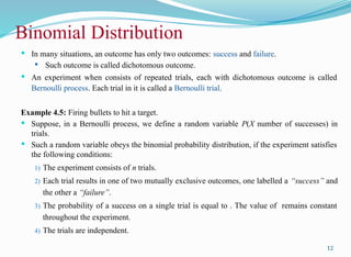
Inmany situations, an outcome has only two outcomes: success and failure.
Such outcome is called dichotomous outcome.
An experiment when consists of repeated trials, each with dichotomous outcome is called
Bernoulli process. Each trial in it is called a Bernoulli trial.
Example 4.5: Firing bullets to hit a target.
Suppose, in a Bernoulli process, we define a random variable P(X number of successes) in
trials.
Such a random variable obeys the binomial probability distribution, if the experiment satisfies
the following conditions:
1) The experiment consists of n trials.
2) Each trial results in one of two mutually exclusive outcomes, one labelled a “success” and
the other a “failure”.
3) The probability of a success on a single trial is equal to . The value of remains constant
throughout the experiment.
4) The trials are independent.
13.
Defining Binomial Distribution
13
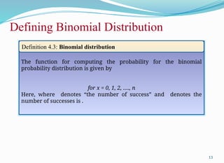
Thefunction for computing the probability for the binomial
probability distribution is given by
for x = 0, 1, 2, …., n
Here, where denotes “the number of success” and denotes the
number of successes is .
Definition 4.3: Binomial distribution
Binomial Distribution
15
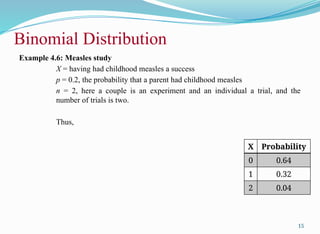
Example 4.6:Measles study
X = having had childhood measles a success
p = 0.2, the probability that a parent had childhood measles
n = 2, here a couple is an experiment and an individual a trial, and the
number of trials is two.
Thus,
X Probability
0 0.64
1 0.32
2 0.04
16.
Binomial Distribution
16
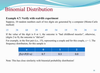
Example 4.7:Verify with real-life experiment
Suppose, 10 random numbers each of two digits are generated by a computer (Monte-Carlo
method)
15 38 68 39 49 54 19 79 38 14
If the value of the digit is 0 or 1, the outcome is “had childhood measles”, otherwise,
(digits 2 to 9), the outcome is “did not”.
For example, in the first pair (i.e., 15), representing a couple and for this couple, x = 1. The
frequency distribution, for this sample is
Note: This has close similarity with binomial probability distribution!
x 0 1 2
f(x)=P(X=x) 0.7 0.3 0.0
17.
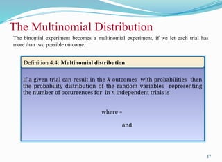
The Multinomial Distribution
17
Ifa given trial can result in the k outcomes with probabilities then
the probability distribution of the random variables representing
the number of occurrences for in n independent trials is
where =
and
Definition 4.4: Multinomial distribution
The binomial experiment becomes a multinomial experiment, if we let each trial has
more than two possible outcome.
18.
The Hypergeometric Distribution
18
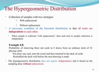
•Collection of samples with two strategies
• With replacement
• Without replacement
• A necessary condition of the binomial distribution is that all trials are
independent to each other.
• When sample is collected “with replacement”, then each trial in sample collection is
independent.
Example 4.8:
Probability of observing three red cards in 5 draws from an ordinary deck of 52
playing cards.
You draw one card, note the result and then returned to the deck of cards
Reshuffled the deck well before the next drawing is made
• The hypergeometric distribution does not require independence and is based on the
sampling done without replacement.
19.
The Hypergeometric Distribution
19
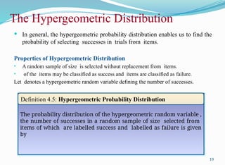
In general, the hypergeometric probability distribution enables us to find the
probability of selecting successes in trials from items.
Properties of Hypergeometric Distribution
• A random sample of size is selected without replacement from items.
• of the items may be classified as success and items are classified as failure.
Let denotes a hypergeometric random variable defining the number of successes.
The probability distribution of the hypergeometric random variable ,
the number of successes in a random sample of size selected from
items of which are labelled success and labelled as failure is given
by
Definition 4.5: Hypergeometric Probability Distribution
20.
Multivariate Hypergeometric Distribution
20
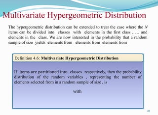
Thehypergeometric distribution can be extended to treat the case where the N
items can be divided into classes with elements in the first class , … and
elements in the class. We are now interested in the probability that a random
sample of size yields elements from elements from elements from
If items are partitioned into classes respectively, then the probability
distribution of the random variables , representing the number of
elements selected from in a random sample of size , is
with
Definition 4.6: Multivariate Hypergeometric Distribution
21.
The Poisson Process
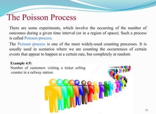
Thereare some experiments, which involve the occurring of the number of
outcomes during a given time interval (or in a region of space). Such a process
is called Poisson process.
The Poisson process is one of the most widely-used counting processes. It is
usually used in scenarios where we are counting the occurrences of certain
events that appear to happen at a certain rate, but completely at random
21
Example 4.9:
Number of customers visiting a ticket selling
counter in a railway station.
22.
The Poisson Process
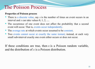
Propertiesof Poisson process
There is a discrete value, say x is the number of times an event occurs in an
interval and x can take values 0, 1, 2, ....
The occurrence of one event does not affect the probability that a second
event will occur. That is, events occur independently.
The average rate at which events occur assumed to be constant.
Two events cannot occur at exactly the same instant; instead, at each very
small sub-interval exactly one event either occurs or does not occur.
If these conditions are true, then x is a Poisson random variable,
and the distribution of x is a Poisson distribution.
22
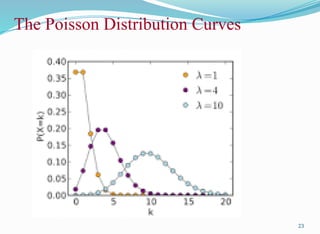
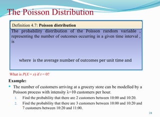
The Poisson Distribution
Example:
The number of customers arriving at a grocery store can be modelled by a
Poisson process with intensity λ=10 customers per hour.
1. Find the probability that there are 2 customers between 10:00 and 10:20.
2. Find the probability that there are 3 customers between 10:00 and 10:20 and
7 customers between 10:20 and 11:00.
24
The probability distribution of the Poisson random variable ,
representing the number of outcomes occurring in a given time interval ,
is
where is the average number of outcomes per unit time and
Definition 4.7: Poisson distribution
What is P(X = x) if t = 0?
25.
Given a randomvariable X in an experiment, we have denoted the probability that .
For discrete events for all values of except
Properties of discrete probability distribution
1. [ is the mean ]
2. [ is the variance ]
In summation is extended for all possible discrete values of .
Note: For discrete uniform distribution, with
and
25
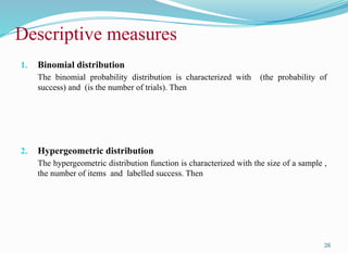
Descriptive measures
26.
1. Binomial distribution
Thebinomial probability distribution is characterized with (the probability of
success) and (is the number of trials). Then
2. Hypergeometric distribution
The hypergeometric distribution function is characterized with the size of a sample ,
the number of items and labelled success. Then
26
Descriptive measures
27.
27
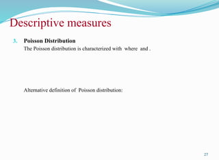
Descriptive measures
3. PoissonDistribution
The Poisson distribution is characterized with where and .
Alternative definition of Poisson distribution:
28.
28
Special Case: DiscreteUniform Distribution
Discrete uniform distribution
A random variable X has a discrete uniform distribution if each of the n values in the
range, say x1, x2, x3, …, xn has equal probability. That is
Where f(x) represents the probability mass function.
Mean and variance for discrete uniform distribution
Suppose, X is a discrete uniform random variable in the range [a,b], such that ab,
then
=
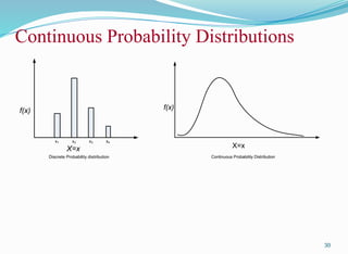
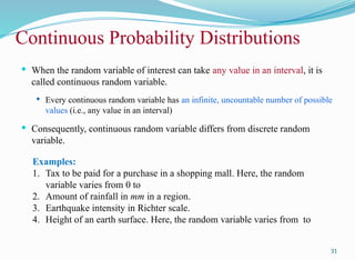
When therandom variable of interest can take any value in an interval, it is
called continuous random variable.
Every continuous random variable has an infinite, uncountable number of possible
values (i.e., any value in an interval)
Consequently, continuous random variable differs from discrete random
variable.
31
Continuous Probability Distributions
Examples:
1. Tax to be paid for a purchase in a shopping mall. Here, the random
variable varies from 0 to
2. Amount of rainfall in mm in a region.
3. Earthquake intensity in Richter scale.
4. Height of an earth surface. Here, the random variable varies from to
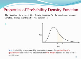
Properties of ProbabilityDensity Function
The function is a probability density function for the continuous random
variable , defined over the set of real numbers , if
1.
33
X=x
f(x)
a b
Note: Probability is represented by area under the curve. The probability of a
specific value of a continuous random variable will be zero because the area under a
point is zero.
34.
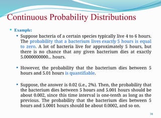
Example:
Supposebacteria of a certain species typically live 4 to 6 hours.
The probability that a bacterium lives exactly 5 hours is equal
to zero. A lot of bacteria live for approximately 5 hours, but
there is no chance that any given bacterium dies at exactly
5.0000000000... hours.
However, the probability that the bacterium dies between 5
hours and 5.01 hours is quantifiable.
Suppose, the answer is 0.02 (i.e., 2%). Then, the probability that
the bacterium dies between 5 hours and 5.001 hours should be
about 0.002, since this time interval is one-tenth as long as the
previous. The probability that the bacterium dies between 5
hours and 5.0001 hours should be about 0.0002, and so on.
34
Continuous Probability Distributions
35.
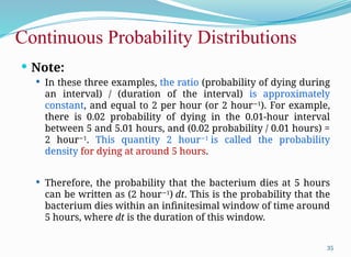
Note:
Inthese three examples, the ratio (probability of dying during
an interval) / (duration of the interval) is approximately
constant, and equal to 2 per hour (or 2 hour 1
−
). For example,
there is 0.02 probability of dying in the 0.01-hour interval
between 5 and 5.01 hours, and (0.02 probability / 0.01 hours) =
2 hour 1
−
. This quantity 2 hour 1
−
is called the probability
density for dying at around 5 hours.
Therefore, the probability that the bacterium dies at 5 hours
can be written as (2 hour 1
−
) dt. This is the probability that the
bacterium dies within an infinitesimal window of time around
5 hours, where dt is the duration of this window.
35
Continuous Probability Distributions
36.
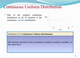
Continuous Uniform Distribution
36
Thedensity function of the continuous uniform random variable on
the interval is:
Definition 4.8: Continuous Uniform Distribution
One of the simplest continuous
distribution in all of statistics is the
continuous uniform distribution. c
A B
f(x)
X=x
37.
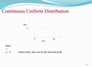
Note:
a)
b) )= whereboth and are in the interval (A,B)
37
Continuous Uniform Distribution
c
A B
f(x)
X=x
38.
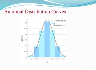
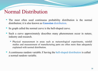
The mostoften used continuous probability distribution is the normal
distribution; it is also known as Gaussian distribution.
Its graph called the normal curve is the bell-shaped curve.
Such a curve approximately describes many phenomenon occur in nature,
industry and research.
Physical measurement in areas such as meteorological experiments, rainfall
studies and measurement of manufacturing parts are often more than adequately
explained with normal distribution.
A continuous random variable X having the bell-shaped distribution is called
a normal random variable.
38
Normal Distribution
39.
39
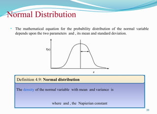
The density ofthe normal variable with mean and variance is
where and , the Napierian constant
Definition 4.9: Normal distribution
Normal Distribution
• The mathematical equation for the probability distribution of the normal variable
depends upon the two parameters and , its mean and standard deviation.
f(x)
x
40.
σ
2
µ1
σ
1
µ2
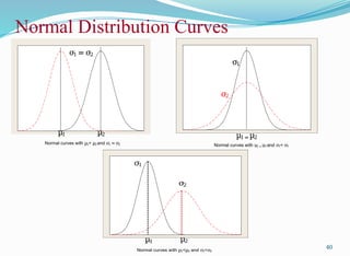
Normal curves withµ1<µ2 and σ
1<σ
2
40
Normal Distribution Curves
µ1 µ2
σ1 = σ2
µ1 µ2
Normal curves with µ1< µ2and σ1 = σ2
σ1
σ2
µ1= µ2
Normal curves with µ1= µ2and σ1< σ2
41.
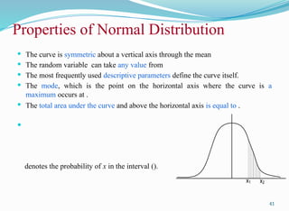
Properties of NormalDistribution
The curve is symmetric about a vertical axis through the mean
The random variable can take any value from
The most frequently used descriptive parameters define the curve itself.
The mode, which is the point on the horizontal axis where the curve is a
maximum occurs at .
The total area under the curve and above the horizontal axis is equal to .
denotes the probability of x in the interval ().
41
x1 x2
42.
The normaldistribution has computational complexity to calculate for any two , and
given and
To avoid this difficulty, the concept of -transformation is followed.
X: Normal distribution with mean and variance .
Z: Standard normal distribution with mean and variance = 1.
Therefore, if f(x) assumes a value, then the corresponding value of is given by
:
=
42
Standard Normal Distribution
[Z-transformation]
43.
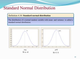
43
Standard Normal Distribution
Thedistribution of a normal random variable with mean and variance is called a
standard normal distribution.
Definition 4.10: Standard normal distribution
3
2
1
0
-1
-2
-3
0.4
0.3
0.2
0.1
0.0
σ=1
25
20
15
10
5
0
-5
0.09
0.08
0.07
0.06
0.05
0.04
0.03
0.02
0.01
0.00
σ
x=µ µ=0
f(x: µ, σ) f(z: 0, 1)
44.
44
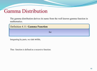
Gamma Distribution
for
Definition 4.11:Gamma Function
The gamma distribution derives its name from the well known gamma function in
mathematics.
Integrating by parts, we can write,
Thus function is defined as a recursive function.
46
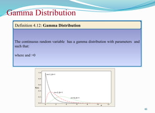
Gamma Distribution
The continuousrandom variable has a gamma distribution with parameters and
such that:
where and >0
Definition 4.12: Gamma Distribution
12
10
8
6
4
2
0
1.0
0.8
0.6
0.4
0.2
0.0
σ
=1,β=1
σ
=2,β=1
σ
=4,β=1
f(x)
x
48
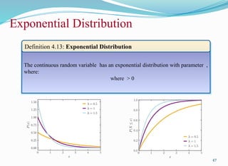
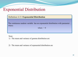
Exponential Distribution
The continuousrandom variable has an exponential distribution with parameter ,
where:
where > 0
Definition 4.13: Exponential Distribution
Note:
1) The mean and variance of gamma distribution are
2) The mean and variance of exponential distribution are
49.
49
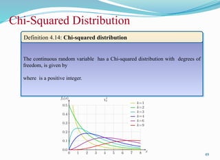
Chi-Squared Distribution
The continuousrandom variable has a Chi-squared distribution with degrees of
freedom, is given by
where is a positive integer.
Definition 4.14: Chi-squared distribution
50.
50
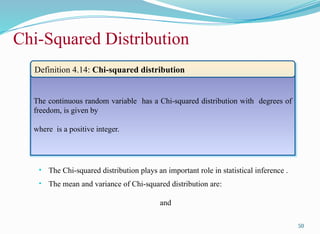
Chi-Squared Distribution
The continuousrandom variable has a Chi-squared distribution with degrees of
freedom, is given by
where is a positive integer.
Definition 4.14: Chi-squared distribution
• The Chi-squared distribution plays an important role in statistical inference .
• The mean and variance of Chi-squared distribution are:
and
51.
51
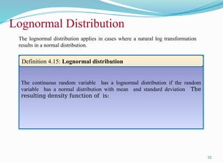
Lognormal Distribution
The continuousrandom variable has a lognormal distribution if the random
variable has a normal distribution with mean and standard deviation The
resulting density function of is:
Definition 4.15: Lognormal distribution
The lognormal distribution applies in cases where a natural log transformation
results in a normal distribution.
53
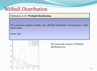
Weibull Distribution
The continuousrandom variable has a Weibull distribution with parameter and
such that.
where and
Definition 4.16: Weibull Distribution
The mean and variance of Weibull
distribution are:
54.
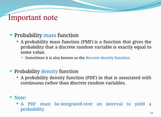
Important note
Probabilitymass function
A probability mass function (PMF) is a function that gives the
probability that a discrete random variable is exactly equal to
some value.
Sometimes it is also known as the discrete density function.
Probability density function
A probability density function (PDF) in that is associated with
continuous rather than discrete random variables.
Note:
A PDF must be integrated over an interval to yield a
probability.
54
56
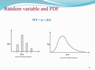
Random variable andPDF
X=x
f(x)
x1 x2 x3 x4
Discrete Probability distribution
X=x
f(x)
Continuous Probability Distribution
P(X = x) = f(x)
57.
In the nextpart of discussion…
Basic concept of sampling distribution
Usage of sampling distributions
Issue with sampling distributions
Central Limit Theorem
Application of Central Limit Theorem
Major sampling distributions
distribution
t-distribution
F distribution
57
58.
58
As a taskof statistical inference, we usually follow the following steps:
Data collection
Collect a sample from the population.
Statistics
Compute a statistics from the sample.
Statistical inference
From the statistics we made various statements concerning the values of population
parameters.
For example, population mean from the sample mean, etc.
Statistical inference
59.
59
Some basic terminologywhich are closely associated to the above-mentioned tasks
are reproduced below.
Population: A population consists of the totality of the observation, with which we are
concerned.
Sample: A sample is a subset of a population.
Random variable: A random variable is a function that associates a real number with
each element in the sample.
Statistics: Any function of the random variable constituting random sample is called a
statistics.
Statistical inference: It is an analysis basically concerned with generalization and
prediction.
Basic terminologies
60.
There are twofacts, which are key to statistical inference.
1. Population parameters are fixed number whose values are usually unknown.
2. Sample statistics are known values for any given sample, but vary from sample to sample, even taken
from the same population.
In fact, it is unlikely for any two samples drawn independently, producing identical values of sample
statistics.
In other words, the variability of sample statistics is always present and must be accounted for in any
inferential procedure.
This variability is called sampling variation.
Note:
A sample statistics is random variable and like any other random variable, a sample statistics has a
probability distribution.
Note: Probability distribution for random variable is not applicable to sample statistics.
60
Statistical learning
61.
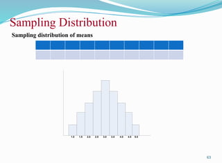
More precisely, samplingdistributions are probability distributions and used to describe
the variability of sample statistics.
The probability distribution of sample mean (hereafter, will be denoted as ) is called
the sampling distribution of the mean (also, referred to as the distribution of sample
mean).
Like we call sampling distribution of variance (denoted as ).
Using the values of and for different random samples of a population, we are to make
inference on the parameters and (of the population).
61
Sampling Distribution
The sampling distribution of a statistics is the probability
distribution of that statistics.
Definition 4.17: Sampling distribution
62.
62
Example 5.1:
Consider fiveidentical balls numbered and weighting as . Consider an experiment consisting of
drawing two balls, replacing the first before drawing the second, and then computing the mean of the
values of the two balls.
Following table lists all possible samples and their mean.
Sampling Distribution
Sample Mean
[1,1]
Sample Mean
[2,4]
Sample Mean
[4,2]
]
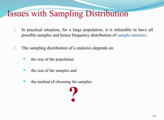
1. In practicalsituation, for a large population, it is infeasible to have all
possible samples and hence frequency distribution of sample statistics.
2. The sampling distribution of a statistics depends on
the size of the population
the size of the samples and
the method of choosing the samples.
64
Issues with Sampling Distribution
?
65.
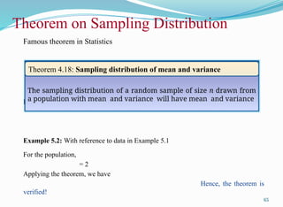
Famous theorem inStatistics
Example: The two balls experiment obeys the theorem.
Example 5.2: With reference to data in Example 5.1
For the population,
= 2
Applying the theorem, we have
Hence, the theorem is
verified!
65
Theorem on Sampling Distribution
The sampling distribution of a random sample of size n drawn from
a population with mean and variance will have mean and variance
Theorem 4.18: Sampling distribution of mean and variance
66.
66
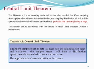
The Theorem 4.1is an amazing result and in fact, also verified that if we sampling
from a population with unknown distribution, the sampling distribution of will still be
approximately normal with mean and variance provided that the sample size is large.
This further, can be established with the famous “Central Limit Theorem”, which is
stated below.
Central Limit Theorem
If random samples each of size are taken from any distribution with mean
and variance , the sample mean will have a distribution
approximately normal with mean and variance .
The approximation becomes better as increases.
Theorem 4.1: Central Limit Theorem
67.
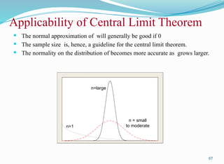
67
The normalapproximation of will generally be good if 0
The sample size is, hence, a guideline for the central limit theorem.
The normality on the distribution of becomes more accurate as grows larger.
Applicability of Central Limit Theorem
n=1
n=large
n = small
to moderate
68.
68
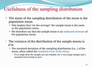
The meanof the sampling distribution of the mean is the
population mean.
This implies that “on the average” the sample mean is the same
as the population mean.
We therefore say that the sample mean is an unbiased estimate of
the population mean.
The variance of the distribution of the sample means is
σ2
/n.
The standard deviation of the sampling distribution (i.e., ) of the
mean, often called the standard error of the mean.
If σ is high then the sample are not reliable, for a very large sample size (,
standard error tends to zero
Usefulness of the sampling distribution
69.
69
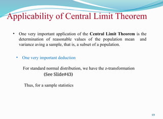
• One veryimportant application of the Central Limit Theorem is the
determination of reasonable values of the population mean and
variance aving a sample, that is, a subset of a population.
• One very important deduction
For standard normal distribution, we have the z-transformation
(See Slide#43)
Thus, for a sample statistics
Applicability of Central Limit Theorem
70.
70
Example:
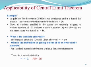
• A quiztest for the course CS61061 was conducted and it is found that
mean of the scores = 90 with standard deviation = 20.
• Now, all students enrolled in the course are randomly assigned to
various sections of 100 students in each. A section (X) was checked and
the mean score was found as = 86.
• What is the standard error rate?
The standard error rate (Central Limit Theorem) = = 2.0
• What is the probability of getting a mean of 86 or lower on the
quiz test?
For standard normal distribution, we have the z-transformation
Thus, for a sample statistics
= = -2. P(Z<-2)?
Applicability of Central Limit Theorem
71.
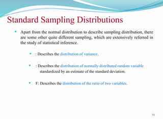
Apart fromthe normal distribution to describe sampling distribution, there
are some other quite different sampling, which are extensively referred in
the study of statistical inference.
: Describes the distribution of variance.
: Describes the distribution of normally distributed random variable
standardized by an estimate of the standard deviation.
F: Describes the distribution of the ratio of two variables.
71
Standard Sampling Distributions
A commonuse of the distribution is to describe the distribution of the sample
variance.
Let X1, X2, . . . , Xn be an independent random variables from a normally
distributed population with mean = μ and variance = σ2
.
The χ2
distribution can be written as
where .
This is also a random variable of a distribution and is called -distribution
(pronounced as Chi-square distribution).
73
The Distribution
74.
74
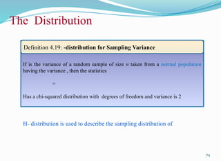
If is thevariance of a random sample of size n taken from a normal population
having the variance , then the statistics
=
Has a chi-squared distribution with degrees of freedom and variance is 2
Definition 4.19: -distribution for Sampling Variance
H- distribution is used to describe the sampling distribution of
The Distribution
75.
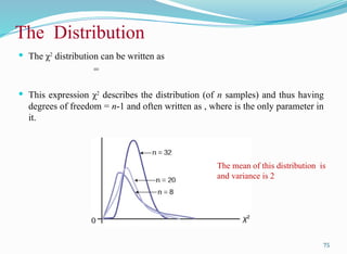
The χ2
distributioncan be written as
=
This expression χ2
describes the distribution (of n samples) and thus having
degrees of freedom = n-1 and often written as , where is the only parameter in
it.
75
The Distribution
The mean of this distribution is
and variance is 2
76.
76
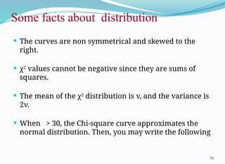
Some facts aboutdistribution
The curves are non symmetrical and skewed to the
right.
χ2
values cannot be negative since they are sums of
squares.
The mean of the χ2
distribution is ν, and the variance is
2ν.
When > 30, the Chi-square curve approximates the
normal distribution. Then, you may write the following
77.
77
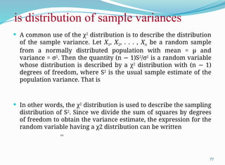
is distribution ofsample variances
A common use of the χ2
distribution is to describe the distribution
of the sample variance. Let X1, X2, . . . , Xn be a random sample
from a normally distributed population with mean = μ and
variance = σ2
. Then the quantity (n 1)S
− 2
/σ2
is a random variable
whose distribution is described by a χ2
distribution with (n 1)
−
degrees of freedom, where S2
is the usual sample estimate of the
population variance. That is
In other words, the χ2
distribution is used to describe the sampling
distribution of S2
. Since we divide the sum of squares by degrees
of freedom to obtain the variance estimate, the expression for the
random variable having a χ2 distribution can be written
=
78.
78
Application of values
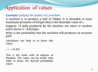
Example:Judging the quality of a machine
A machine is to produce a ball of 100gm. It is desirable to have
maximum deviation of 0.01gm (this is the desirable value of ).
Suppose, 15 balls produced by the machine are select at random
and it shows S = 0.0125gm.
What is the probability that the machine will produces an accurate
ball?
calculation can help us to know this
value.
= = = 21.875
This is the value with 14 degrees of
freedom. The value can be tested with
table to know the desired probability
value.
80
The Distribution
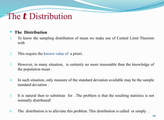
1.To know the sampling distribution of mean we make use of Central Limit Theorem
with
2. This require the known value of a priori.
3. However, in many situation, is certainly no more reasonable than the knowledge of
the population mean .
4. In such situation, only measure of the standard deviation available may be the sample
standard deviation .
5. It is natural then to substitute for . The problem is that the resulting statistics is not
normally distributed!
6. The distribution is to alleviate this problem. This distribution is called or simply .
The Distribution
𝒕
81.
81
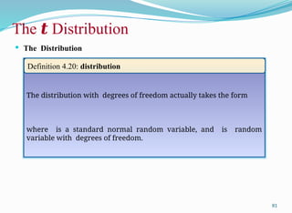
The Distribution
Thedistribution with degrees of freedom actually takes the form
where is a standard normal random variable, and is random
variable with degrees of freedom.
Definition 4.20: distribution
The Distribution
𝒕
82.
82
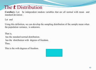
Corollary: Let beindependent random variables that are all normal with mean and
standard deviation .
Let and
Using this definition, we can develop the sampling distribution of the sample mean when
the population variance, is unknown.
That is,
has the standard normal distribution.
has the distribution with degrees of freedom.
Thus,
This is the with degrees of freedom.
The Distribution
𝒕
84
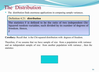
The distributionfinds enormous applications in comparing sample variances.
Corollary: Recall that is the Chi-squared distribution with degrees of freedom.
Therefore, if we assume that we have sample of size from a population with variance
and an independent sample of size from another population with variance , then the
statistics
The Distribution
The statistics F is defined to be the ratio of two independent Chi-
Squared random variables, each divided by its number of degrees of
freedom. Hence,
F
Definition 4.21: distribution
85.
85
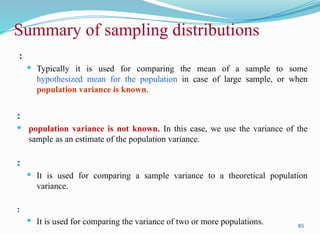
:
Typically itis used for comparing the mean of a sample to some
hypothesized mean for the population in case of large sample, or when
population variance is known.
:
population variance is not known. In this case, we use the variance of the
sample as an estimate of the population variance.
:
It is used for comparing a sample variance to a theoretical population
variance.
:
It is used for comparing the variance of two or more populations.
Summary of sampling distributions
86.
Reference
86
The detailmaterial related to this lecture can be found in
Probability and Statistics for Engineers and Scientists (8th
Ed.)
by Ronald E. Walpole, Sharon L. Myers, Keying Ye (Pearson),
2013.
87.
Questions of theday…
1. Give some examples of random variables? Also, tell the
range of values and whether they are with continuous
or discrete values.
2. In the following cases, what are the probability
distributions are likely to be followed. In each case, you
should mention the random variable and the
parameter(s) influencing the probability distribution
function.
a) In a retail source, how many counters should be opened at a
given time period.
b) Number of people who are suffering from cancers in a town?
87
88.
Questions of theday…
2. In the following cases, what are the probability
distributions are likely to be followed. In each case,
you should mention the random variable and the
parameter(s) influencing the probability distribution
function.
c) A missile will hit the enemy’s aircraft.
d) A student in the class will secure EX grade.
e) Salary of a person in an enterprise.
f) Accident made by cars in a city.
g) People quit education after i) primary ii) secondary and iii)
higher secondary educations.
88
89.
Questions of theday…
3. How you can calculate the mean and standard
deviation of a population if the population follows
the following probability distribution functions with
respect to an event.
a) Binomial distribution function.
b) Poisson’s distribution function.
c) Hypergeometric distribution function.
d) Normal distribution function.
e) Standard normal distribution function.
89
90.
Questions of theday…
4. What are the degrees of freedom in the following
cases.
Case 1: A single number.
Case 2: A list of n numbers.
Case 3: a table of data with m rows and n columns.
Case 4: a data cube with dimension m×n×p.
90
91.
Questions of theday…
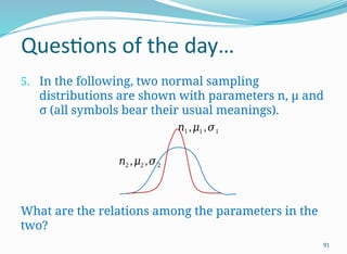
5. In the following, two normal sampling
distributions are shown with parameters n, μ and
σ (all symbols bear their usual meanings).
What are the relations among the parameters in the
two?
91
𝑛1 ,𝜇1 ,𝜎1
𝑛2 ,𝜇2 ,𝜎2
92.
Questions of theday…
6. Suppose, and S denote the sample mean and
standard deviation of a sample. Assume that
population follows normal distribution with
population mean and standard deviation . Write
down the expression of z and t values with
degree of freedom n.
92

![Given a random variable X in an experiment, we have denoted the probability that .
For discrete events for all values of except
Properties of discrete probability distribution
1. [ is the mean ]
2. [ is the variance ]
In summation is extended for all possible discrete values of .
Note: For discrete uniform distribution, with
and
25
Descriptive measures](https://image.slidesharecdn.com/04staisticalmethods-250215051010-be3dfe90/85/Predictive-analytics-using-R-Programming-25-320.jpg)
![28
Special Case: Discrete Uniform Distribution
Discrete uniform distribution
A random variable X has a discrete uniform distribution if each of the n values in the
range, say x1, x2, x3, …, xn has equal probability. That is
Where f(x) represents the probability mass function.
Mean and variance for discrete uniform distribution
Suppose, X is a discrete uniform random variable in the range [a,b], such that ab,
then
=](https://image.slidesharecdn.com/04staisticalmethods-250215051010-be3dfe90/85/Predictive-analytics-using-R-Programming-28-320.jpg)
![ The normal distribution has computational complexity to calculate for any two , and
given and
To avoid this difficulty, the concept of -transformation is followed.
X: Normal distribution with mean and variance .
Z: Standard normal distribution with mean and variance = 1.
Therefore, if f(x) assumes a value, then the corresponding value of is given by
:
=
42
Standard Normal Distribution
[Z-transformation]](https://image.slidesharecdn.com/04staisticalmethods-250215051010-be3dfe90/85/Predictive-analytics-using-R-Programming-42-320.jpg)
![45
Gamma Distribution
When , we can write,
!
Further,
Note:
[An important property]](https://image.slidesharecdn.com/04staisticalmethods-250215051010-be3dfe90/85/Predictive-analytics-using-R-Programming-45-320.jpg)

![62
Example 5.1:
Consider five identical balls numbered and weighting as . Consider an experiment consisting of
drawing two balls, replacing the first before drawing the second, and then computing the mean of the
values of the two balls.
Following table lists all possible samples and their mean.
Sampling Distribution
Sample Mean
[1,1]
Sample Mean
[2,4]
Sample Mean
[4,2]
]](https://image.slidesharecdn.com/04staisticalmethods-250215051010-be3dfe90/85/Predictive-analytics-using-R-Programming-62-320.jpg)