Concepts Covered
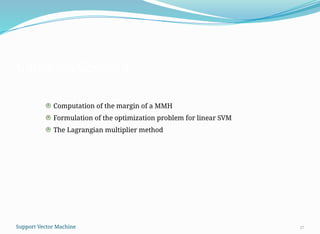
2
Introduction toSVM
Concept of Maximum Margin Hyperplane (MMH)
Computation of the margin of a MMH
Formulation of the optimization problem for linear SVM
The Lagrangian multiplier method
Building model for linear SVM
Multiclass classification
Non-linear SVM
Concept of non-linear data
Φ-transformation
Dual formation of optimization problem
Kernel tricks and kernel functions
Plan of the lectures
Support Vector Machine
Support Vector Machine
4
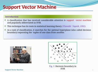
Aclassification that has received considerable attention is support vector machine
and popularly abbreviated as SVM.
This technique has its roots in statistical learning theory (Vlamidir Vapnik, 1992).
As a task of classification, it searches for the optimal hyperplane (also called decision
boundary) separating the tuples of one class from another.
Introduction
Fig. 1: Decision boundary in
SVM
Support Vector Machine
5.
Support Vector Machine
5
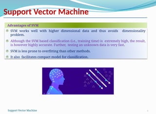
SVMworks well with higher dimensional data and thus avoids dimensionality
problem.
Although the SVM based classification (i.e., training time) is extremely high, the result,
is however highly accurate. Further, testing an unknown data is very fast.
SVM is less prone to overfitting than other methods.
It also facilitates compact model for classification.
Advantages of SVM
Support Vector Machine
6.
Overfitting and UnderfittingIssues
6
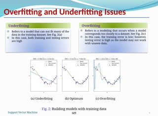
Underfitting
Refers to a model that can not fit many of the
data in the training dataset. See Fig. 2(a)
In this case, both training and testing errors
are high
Overfitting
Refers to a modeling that occurs when a model
corresponds too closely to a dataset. See Fig. 2(c)
In this case, the training error is low; however,
testing error is high as the model may not work
with unseen data.
Fig. 2: Building models with training data
set
(a) Underfitting (c) Overfitting
(b) Optimum
Support Vector Machine
7.
Support Vector Machines
7
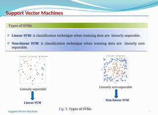
LinearSVM: A classification technique when training data are linearly separable.
Non-linear SVM: A classification technique when training data are linearly non-
separable.
Types of SVMs
Linearly separable
Linearly non-separable
Linear SVM
Non-linear SVM
Fig. 3: Types of SVMs
Support Vector Machine
Decision Boundaries
9
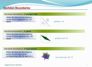
When thedata are described in
terms of two attributes (i.e., 2D
data).
Decision boundary: A straight line
When the data are described in
terms of three attributes (i.e., 3D
data)
Decision boundary: A plane
When the data are described in
terms of more than three
attributes (e.g., 4D, 5D, data, etc.).
Decision boundary: A hyperplane
ax+by+c = 0
ax+by+cz+d = 0
a1x1+a2x2+a3x3++b = 0
Support Vector Machine
10.
Classification Problem
10
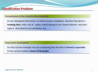
In oursubsequent discussion, we shall assume a simplistic situation that given a
training data with a set of tuples, which belong to two classes eitheror and each
tuple is described by two attributes, say .
Formulation of the classification problem
For this current example, we are considering that the data is linearly separable.
So the current model is linear SVM model.
Important Assumption
Support Vector Machine
11.
Classification with Hyperplane
11
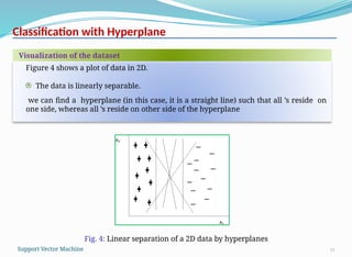
Figure4 shows a plot of data in 2D.
The data is linearly separable.
we can find a hyperplane (in this case, it is a straight line) such that all ’s reside on
one side, whereas all ’s reside on other side of the hyperplane
Visualization of the dataset
Fig. 4: Linear separation of a 2D data by hyperplanes
Support Vector Machine
12.
Classification with Hyperplane
12
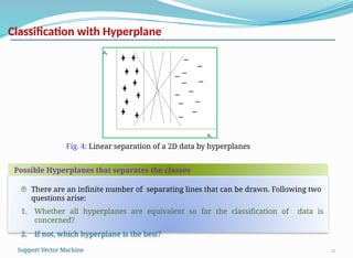
Thereare an infinite number of separating lines that can be drawn. Following two
questions arise:
1. Whether all hyperplanes are equivalent so far the classification of data is
concerned?
2. If not, which hyperplane is the best?
Possible Hyperplanes that separates the classes
Fig. 4: Linear separation of a 2D data by hyperplanes
Support Vector Machine
13.
Classification with Hyperplane
13
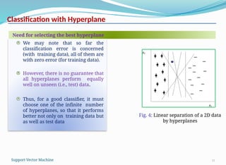
Wemay note that so far the
classification error is concerned
(with training data), all of them are
with zero error (for training data).
However, there is no guarantee that
all hyperplanes perform equally
well on unseen (i.e., test) data.
Thus, for a good classifier, it must
choose one of the infinite number
of hyperplanes, so that it performs
better not only on training data but
as well as test data
Need for selecting the best hyperplane
Fig. 4: Linear separation of a 2D data
by hyperplanes
Support Vector Machine
14.
Classification with Hyperplane
14
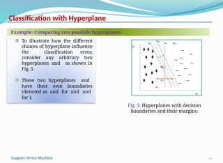
Toillustrate how the different
choices of hyperplane influence
the classification error,
consider any arbitrary two
hyperplanes and as shown in
Fig. 5
These two hyperplanes and
have their own boundaries
(denoted as and for and and
for ).
Example: Comparing two possible hyperplanes
Fig. 5: Hyperplanes with decision
boundaries and their margins.
m2
Support Vector Machine
15.
Hyperplane and Margin
15
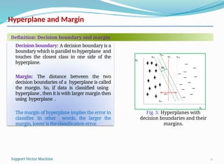
Decisionboundary: A decision boundary is a
boundary which is parallel to hyperplane and
touches the closest class in one side of the
hyperplane.
Margin: The distance between the two
decision boundaries of a hyperplane is called
the margin. So, if data is classified using
hyperplane , then it is with larger margin then
using hyperplane .
The margin of hyperplane implies the error in
classifier. In other words, the larger the
margin, lower is the classification error.
Definition: Decision boundary and margin
Fig. 5: Hyperplanes with
decision boundaries and their
margins.
m2
Support Vector Machine
16.
Maximum Margin Hyperplane
16
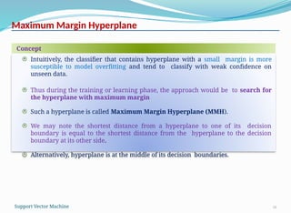
Intuitively,the classifier that contains hyperplane with a small margin is more
susceptible to model overfitting and tend to classify with weak confidence on
unseen data.
Thus during the training or learning phase, the approach would be to search for
the hyperplane with maximum margin
Such a hyperplane is called Maximum Margin Hyperplane (MMH).
We may note the shortest distance from a hyperplane to one of its decision
boundary is equal to the shortest distance from the hyperplane to the decision
boundary at its other side.
Alternatively, hyperplane is at the middle of its decision boundaries.
Concept
Support Vector Machine
Linear SVM
18
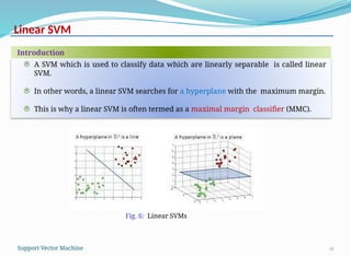
A SVMwhich is used to classify data which are linearly separable is called linear
SVM.
In other words, a linear SVM searches for a hyperplane with the maximum margin.
This is why a linear SVM is often termed as a maximal margin classifier (MMC).
Introduction
Fig. 6: Linear SVMs
Support Vector Machine
19.
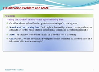
Classification Problem andMMH
19
Finding the MMH for linear SVM for a given training data:
Consider a binary classification problem consisting of n training data
Notation of the training data: Each tuple is denoted by where corresponds to the
attribute set for the tuple (data in dimensional space) and denotes its class label
Note: The choice of which class should be labeled as or is arbitrary
Goal: Given , we are to obtain a hyperplane which separates all into two sides of it
(of course with maximum margin)
Notations
Support Vector Machine
20.
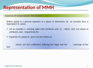
Representation of MMH
20
Before,going to a general equation of a plane in dimension, let us consider first, a
hyperplane in plane.
Let us consider a training tuple with attributes and as , where and are values of
attributes and , respectively for
Equation of a plane in space can be written as
where, are the coefficients defining the slope and the intercept of the
line
Equation of a hyperplane: The 2D case
Support Vector Machine
21.
MMH and Classification
21
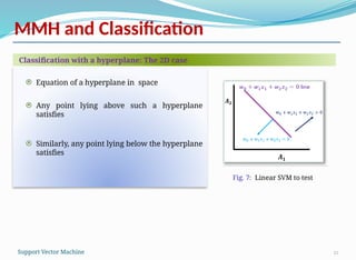
Equationof a hyperplane in space
Any point lying above such a hyperplane
satisfies
Similarly, any point lying below the hyperplane
satisfies
Classification with a hyperplane: The 2D case
Fig. 7: Linear SVM to test
Support Vector Machine
22.
Representation of MMH
22
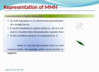
AnSVM hyperplane is an dimensional generalization
of a straight line in .
It can be visualized as a plane surface in , but it is not
easy to visualize when dimensionality is greater than
In fact, Euclidean equation of a hyperplane in is
where wi ’s are the real numbers and b is a real
constant (called the intercept, which can be positive or
negative).
Generalization to higher dimensions
Support Vector Machine
23.
Representation of MMH
23
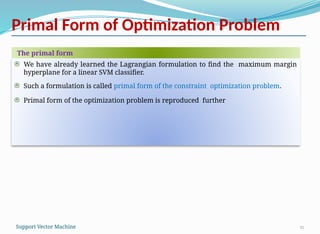
Inmatrix form, a hyperplane can be represented as
where and and b is a real constant.
Here, W and b are parameters of the classifier model to be
learned given a training data set D
Equation of a hyperplane in matrix form
[
𝑥1
𝑥2
∙
∙
∙
𝑥𝑚
]
Support Vector Machine
24.
Margin of MMH
24
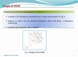
Considera 2D training set consisting of two classes and as shown in Fig. 8
Suppose, b1 and b2 are two decision boundaries above and below a hyperplane,
respectively
Consider any two points and as shown
Finding the margin of a hyperplane
Fig. 8: Margin of the MMH
Support Vector Machine
25.
Margin of MMH
25
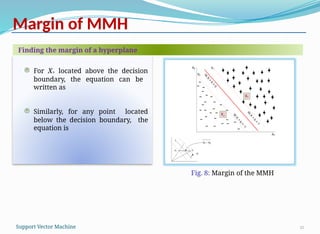
ForX+ located above the decision
boundary, the equation can be
written as
Similarly, for any point located
below the decision boundary, the
equation is
Finding the margin of a hyperplane
Fig. 8: Margin of the MMH
Support Vector Machine
26.
Margin of MMH
26
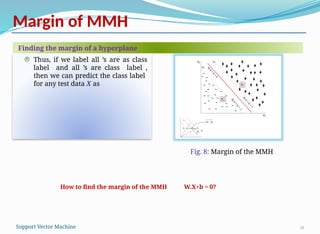
Thus,if we label all ’s are as class
label and all ’s are class label ,
then we can predict the class label
for any test data X as
Finding the margin of a hyperplane
Fig. 8: Margin of the MMH
How to find the margin of the MMH W.X+b = 0?
Support Vector Machine
27.
Concepts Covered
27
Computation ofthe margin of a MMH
Formulation of the optimization problem for linear SVM
The Lagrangian multiplier method
Support Vector Machine
MMH for LinearSVM
29
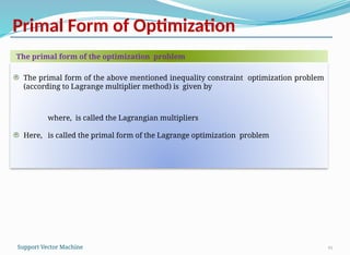
We learnt,
The equation of the hyperplane
in matrix form is:
where and and b is a real
constant.
Thus, if we label all ’s are as
class label and all ’s are
class label , then we can
predict the class label for
any test data X as
RECAP: Equation of the hyperplane in matrix form
Fig. 8: Margin of the MMH
[
𝑥1
𝑥2
∙
∙
∙
𝑥𝑚
]
Support Vector Machine
30.
Computation of marginof MMH
30
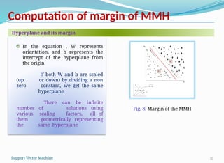
In the equation , W represents
orientation, and b represents the
intercept of the hyperplane from
the origin
If both W and b are scaled
(up or down) by dividing a non
zero constant, we get the same
hyperplane
There can be infinite
number of solutions using
various scaling factors, all of
them geometrically representing
the same hyperplane
Hyperplane and its margin
Fig. 8: Margin of the MMH
Support Vector Machine
31.
Margin of MMH
31
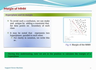
Toavoid such a confusion, we can make
and unique by adding a constraint that
for data points on boundary of each
class
It may be noted that represents two
hyperplanes parallel to each other.
For clarity in notation, we write this
as .
Hyperplane and its margin
Having this understating, now we are in the position to calculate the margin of a
hyperplane
Fig. 8: Margin of the MMH
Support Vector Machine
32.
Computation of Marginof a MMH
32
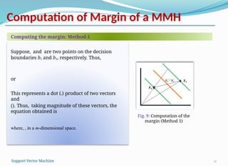
Suppose, and are two points on the decision
boundaries b1 and b2, respectively. Thus,
or
This represents a dot (.) product of two vectors
and
(). Thus, taking magnitude of these vectors, the
equation obtained is
where, , in a m-dimensional space.
Computing the margin: Method-1
Fig. 9: Computation of the
margin (Method 1)
Support Vector Machine
33.
Computation of Marginof a MMH
33
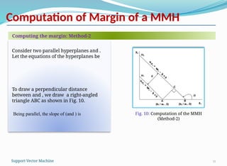
Consider two parallel hyperplanes and .
Let the equations of the hyperplanes be
To draw a perpendicular distance
between and , we draw a right-angled
triangle ABC as shown in Fig. 10.
Being parallel, the slope of (and ) is
Computing the margin: Method-2
Fig. 10: Computation of the MMH
(Method-2)
Support Vector Machine
34.
Computation of Marginof a MMH
34
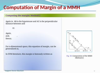
Again in AB is the hypotenuse and AC is the perpendicular
distance between and
or,
Again,
and, ,
Hence,
For n-dimensional space, this equation of margin, can be
generalized as,
In SVM literature, this margin is famously written as
Computing the margin: Method-2
Fig. 10: Computation of the MMH
(Method-2)
Support Vector Machine
Finding MMH ofa SVM
36
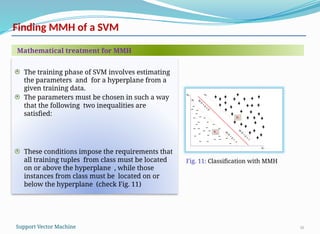
The training phase of SVM involves estimating
the parameters and for a hyperplane from a
given training data.
The parameters must be chosen in such a way
that the following two inequalities are
satisfied:
These conditions impose the requirements that
all training tuples from class must be located
on or above the hyperplane , while those
instances from class must be located on or
below the hyperplane (check Fig. 11)
Fig. 11: Classification with MMH
Mathematical treatment for MMH
Support Vector Machine
37.
Computing MMH ofa SVM
37
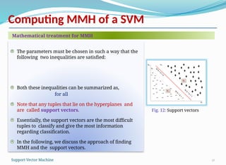
The parameters must be chosen in such a way that the
following two inequalities are satisfied:
Both these inequalities can be summarized as,
for all
Note that any tuples that lie on the hyperplanes and
are called support vectors.
Essentially, the support vectors are the most difficult
tuples to classify and give the most information
regarding classification.
In the following, we discuss the approach of finding
MMH and the support vectors.
Fig. 12: Support vectors
Mathematical treatment for MMH
Support Vector Machine
38.
Computing MMH ofa SVM
38
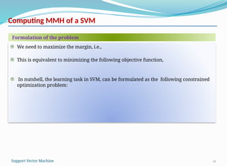
We need to maximize the margin, i.e.,
This is equivalent to minimizing the following objective function,
In nutshell, the learning task in SVM, can be formulated as the following constrained
optimization problem:
Formulation of the problem
Support Vector Machine
39.
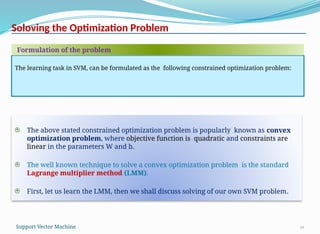
Soloving the OptimizationProblem
39
The above stated constrained optimization problem is popularly known as convex
optimization problem, where objective function is quadratic and constraints are
linear in the parameters W and b.
The well known technique to solve a convex optimization problem is the standard
Lagrange multiplier method (LMM).
First, let us learn the LMM, then we shall discuss solving of our own SVM problem.
The learning task in SVM, can be formulated as the following constrained optimization problem:
Formulation of the problem
Support Vector Machine
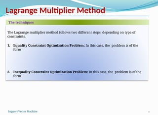
Lagrange Multiplier Method
41
TheLagrange multiplier method follows two different steps depending on type of
constraints.
1. Equality Constraint Optimization Problem: In this case, the problem is of the
form
2. Inequality Constraint Optimization Problem: In this case, the problem is of the
form
The techniques
Support Vector Machine
42.
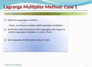
Lagrange Multiplier Method:Case 1
42
1) Define the Lagrangian as follows:
L =
where, are dummy variables called Lagrangian multipliers
2) Set the first order derivatives of the Lagrangian with respect to
and the Lagrangian multipliers to zero’s. That is
3) Solve equations to find optimal value of and s
Case 1: Equality constraint optimization problem solving
Support Vector Machine
43.
Lagrange Multiplier Method:Case 1
43
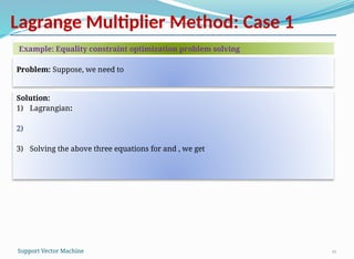
Problem: Suppose, we need to
Example: Equality constraint optimization problem solving
Solution:
1) Lagrangian:
2)
3) Solving the above three equations for and , we get
Support Vector Machine
44.
Lagrange Multiplier Method:Case 1
44
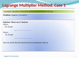
Problem: Suppose, we need to
Example: Equality constraint optimization problem solving
Solution: There are 23
choices:
When, ,
So, we get
… . . . . . . . . . . .
When, ,
So, we get
… . . . . . . . . . . .
You can check that the function has its minimum value at
Support Vector Machine
45.
Lagrange Multiplier Method:Case 2
45
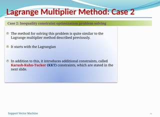
The method for solving this problem is quite similar to the
Lagrange multiplier method described previously.
It starts with the Lagrangian
In addition to this, it introduces additional constraints, called
Karush-Kuhn-Tucker (KKT) constraints, which are stated in the
next slide.
Case 2: Inequality constraint optimization problem solving
Support Vector Machine
46.
Lagrange Multiplier Method:Case 2
46
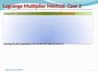
Solving the above equations, we can find the optimal value of
Inequality constraint optimization problem solving: KKT constraints
Support Vector Machine
47.
Lagrange Multiplier Method:Case 2
47
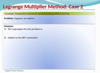
Problem: Suppose, we need to
Example: Inequality constraint optimization problem solving
Solution:
1) The Lagrangian for this problem is
2) Subject to the KKT constraints:
Support Vector Machine
48.
Lagrange Multiplier Method:Case 2
48
Example: Inequality constraint optimization problem solving
Solution:
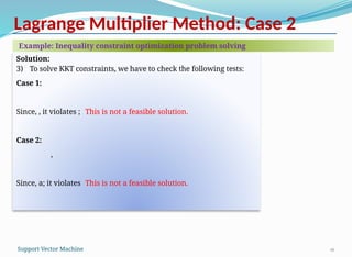
3) To solve KKT constraints, we have to check the following tests:
Case 1:
Since, , it violates ; This is not a feasible solution.
Case 2:
,
Since, a; it violates This is not a feasible solution.
Support Vector Machine
49.
Lagrange Multiplier Method:Case 2
49
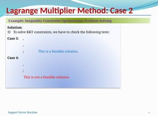
Example: Inequality Constraint Optimization Problem Solving
Solution:
3) To solve KKT constraints, we have to check the following tests:
Case 3: ,
,
; This is a feasible solution.
Case 4:
,
;
This is not a feasible solution.
Support Vector Machine
50.
50
Concepts Covered
Obtaining thehyperplane using Lagrangian multiplier method
Multiclass classification using linear SVM
Support Vector Machine
52
LMM to SolveLinear SVM
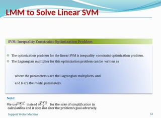
The optimization problem for the linear SVM is inequality constraint optimization problem.
The Lagrangian multiplier for this optimization problem can be written as
where the parameters s are the Lagrangian multipliers, and
and b are the model parameters.
‖𝑊‖
2
2
Note:
We use instead of for the sake of simplification in
calculations and it does not alter the problem’s goal adversely.
‖𝑊‖
2
SVM: Inequality Constraint Optimization Problem
Support Vector Machine
53.
53
LMM to SolveLinear SVM
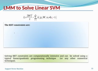
The KKT constraints are:
,
Solving KKT constraints are computationally intensive and can be solved using a
typical linear/quadratic programming technique (or any other numerical
technique).
𝐿=
‖𝑊‖
2
2
−∑
𝑖=1
𝑛
𝜆𝑖 (𝑦𝑖 (𝑊 .𝑥𝑖+𝑏¿−1))
Support Vector Machine
54.
54
Note:
LMM to SolveLinear SVM
We first solve the above set of equations to find all the feasible solutions.
Then, we can determine optimum value of .
Lagrangian multiplier must be zero unless the training instance satisfies the
equation .
Thus, the training tuples with lie on the hyperplane margins and hence are support
vectors.
The training instances that do not lie on the hyperplane margin have .
Support Vector Machine
55.
55
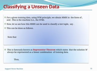
For a giventraining data, using SVM principle, we obtain MMH in the form of ,
and . This is the machine (i.e., the SVM).
Now, let us see how this MMH can be used to classify a test tuple, say .
This can be done as follows.
Note that
Classifying a Unseen Data
This is famously known as Representor Theorem which states that the solution W
always be represented as a linear combination of training data.
Thus,
Support Vector Machine
56.
56
Note:
Classifying a UnseenData
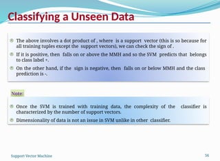
The above involves a dot product of , where is a support vector (this is so because for
all training tuples except the support vectors), we can check the sign of .
If it is positive, then falls on or above the MMH and so the SVM predicts that belongs
to class label +.
On the other hand, if the sign is negative, then falls on or below MMH and the class
prediction is -.
Once the SVM is trained with training data, the complexity of the classifier is
characterized by the number of support vectors.
Dimensionality of data is not an issue in SVM unlike in other classifier.
Support Vector Machine
57.
57
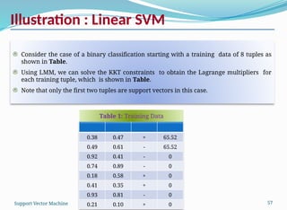
Illustration : LinearSVM
Consider the case of a binary classification starting with a training data of 8 tuples as
shown in Table.
Using LMM, we can solve the KKT constraints to obtain the Lagrange multipliers for
each training tuple, which is shown in Table.
Note that only the first two tuples are support vectors in this case.
0.38 0.47 + 65.52
0.49 0.61 - 65.52
0.92 0.41 - 0
0.74 0.89 - 0
0.18 0.58 + 0
0.41 0.35 + 0
0.93 0.81 - 0
0.21 0.10 + 0
Table 1: Training Data
Support Vector Machine
58.
58
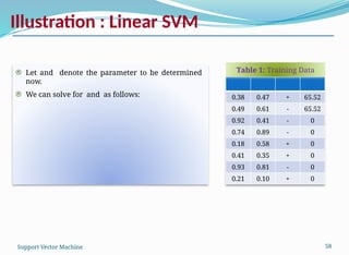
Illustration : LinearSVM
Let and denote the parameter to be determined
now.
We can solve for and as follows: 0.38 0.47 + 65.52
0.49 0.61 - 65.52
0.92 0.41 - 0
0.74 0.89 - 0
0.18 0.58 + 0
0.41 0.35 + 0
0.93 0.81 - 0
0.21 0.10 + 0
Table 1: Training Data
Support Vector Machine
59.
59
Illustration : LinearSVM
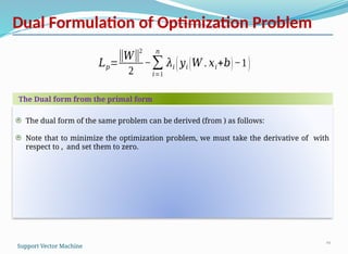
The parameter can be calculated for each support vector as follows
// for support vector
//using dot product
// for support vector
//using dot product
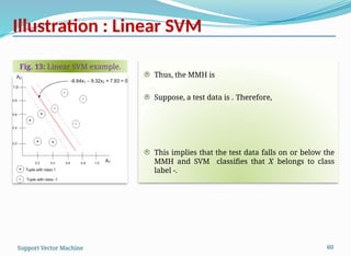
Averaging these values of and , we get .
W = [-6.64 -9.32]
x1 = [0.38 0.47]
x2 = [0.49 0.61]
Support Vector Machine
60.
60
Illustration : LinearSVM
Fig. 13: Linear SVM example.
Thus, the MMH is
Suppose, a test data is . Therefore,
This implies that the test data falls on or below the
MMH and SVM classifies that X belongs to class
label -.
Support Vector Machine
62
Classification of Multiple-classData
In the discussion of linear SVM, we have limited our discussion to binary
classification (i.e., classification with two classes only).
Note that the discussed linear SVM can handle any n-dimension, .
Now, we are to discuss a more generalized linear SVM to classify n-dimensional data
belong to two or more classes.
There are two possibilities:
all classes are pairwise linearly separable, or
all classes are overlapping (not linearly separable.)
Support Vector Machine
63.
63
Classification of Multiple-classData
If the classes are pair-wise linearly separable, then we can extend the principle of
linear SVM to each pair.
There are two strategies:
One versus one (OVO) strategy
One versus all (OVA) strategy
Support Vector Machine
64.
64
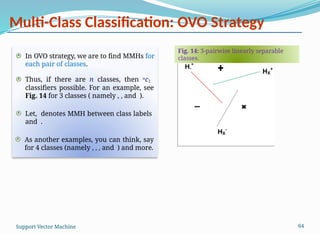
Multi-Class Classification: OVOStrategy
In OVO strategy, we are to find MMHs for
each pair of classes.
Thus, if there are n classes, then nc2
classifiers possible. For an example, see
Fig. 14 for 3 classes ( namely , , and ).
Let, denotes MMH between class labels
and .
As another examples, you can think, say
for 4 classes (namely , , , and ) and more.
Fig. 14: 3-pairwise linearly separable
classes.
Support Vector Machine
65.
65
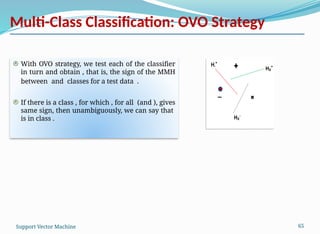
Multi-Class Classification: OVOStrategy
With OVO strategy, we test each of the classifier
in turn and obtain , that is, the sign of the MMH
between and classes for a test data .
If there is a class , for which , for all (and ), gives
same sign, then unambiguously, we can say that
is in class .
Support Vector Machine
66.
66
Multi-Class Classification: OVAStrategy
OVO strategy is not useful for data with a large number of classes, as the
computational complexity increases exponentially with the number of classes.
As an alternative to OVO strategy, OVA(One Versus All) strategy has been proposed.
In this approach, we choose any class say and consider that all tuples of other classes
belong to a single class.
Support Vector Machine
67.
67
Multi-Class Classification: OVAStrategy
This is, therefore, transformed into a binary classification problem and using the
linear SVM discussed above, we can find the hyperplane.
Let the hyperplane between and remaining classes be .
The process is repeated for each and getting s
In other words, with OVA strategies we get classifiers.
Support Vector Machine
68.
68
Note:
Multi-Class Classification: OVAStrategy
The linear SVM that is used to classify multi-class data fails, if all classes are not
linearly separable.
If one class is linearly separable to remaining other classes and test data belongs to
that particular class, then only it classifies accurately.
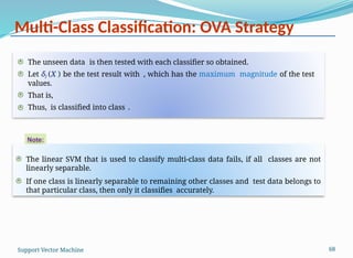
The unseen data is then tested with each classifier so obtained.
Let δj (X ) be the test result with , which has the maximum magnitude of the test
values.
That is,
Thus, is classified into class .
Support Vector Machine
69.
69
Multi-Class Classification: OVAStrategy
Further, it is possible to have some tuples which cannot be classified to any of the
linear SVMs.
There are some tuples which cannot be classified unambiguously by neither of the
hyperplanes.
All these tuples may be due to noise, errors or data are not linearly separable.
Fig. 15: Unclassifiable region in OVA strategy.
Support Vector Machine
72
Non-linear SVM
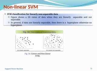
SVM classificationfor linearly non-separable data
Figure shows a 2D views of data when they are linearly separable and not
separable.
In general, if data are linearly separable, then there is a hyperplane otherwise no
hyperplane.
Fig. 16: Two types of training data.
Fig. 16: Linear and Non-linear
SVMs
Support Vector Machine
73.
73
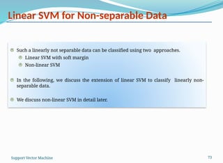
Linear SVM forNon-separable Data
Such a linearly not separable data can be classified using two approaches.
Linear SVM with soft margin
Non-linear SVM
In the following, we discuss the extension of linear SVM to classify linearly non-
separable data.
We discuss non-linear SVM in detail later.
Support Vector Machine
74.
74
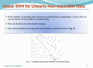
If the numberof training data instances violating linear separability is less, then we
can use linear SVM classifier to classify them.
This can be done by reducing the margin
The rational behind this approach can be better understood from Fig. 17.
Linear SVM for Linearly Non-separable Data
Fig. 17: Problem with linear SVM for non-linear data
Support Vector Machine
75.
75
Non-Linear SVM
Linear SVMundoubtedly better to classify data if it is trained by linearly separable
data.
Linear SVM also can be used for non-linearly separable data, provided that number
of such instances is less.
However, in real life applications, number of data overlapping is so high that the
approach cannot cope to yield accurate classifier.
As an alternative to this there is a need to compute a decision boundary, which is not
linear (i.e., not a hyperplane rather hypersurface).
Support Vector Machine
76.
76
Non-Linear SVM
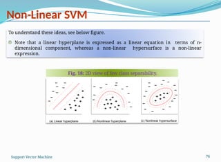
To understandthese ideas, see below figure.
Note that a linear hyperplane is expressed as a linear equation in terms of n-
dimensional component, whereas a non-linear hypersurface is a non-linear
expression.
Fig. 18: 2D view of few class separability.
Support Vector Machine
77.
77
Non-Linear SVM
A hyperplaneis expressed as
Whereas a non-linear hypersurface is expressed as.
The task therefore takes a turn to find a nonlinear decision boundaries, that is, a
nonlinear hypersurface in input space comprising with linearly non separable data.
This task indeed neither hard nor so complex, and fortunately can be accomplished
extending the formulation of linear SVM, we have already learned.
Support Vector Machine
78.
78
Non-Linear SVM
This canbe achieved in two major steps.
Transform the original (non-linear) input data into a higher dimensional
space (as a linear representation of data).
Note that this is feasible because SVM’s performance is decided by number
of support vectors (i.e., training data
≈ ) not by the dimension of data.
Search for the linear decision boundaries to separate the transformed
higher dimensional data.
The above can be done in the same line as we have done for linear SVM.
Support Vector Machine
79.
79
Concept of Non-LinearMapping
In nutshell, to have a nonlinear SVM, the trick is to transform non-linear data
into higher dimensional linear data.
This transformation is popularly called non-linear mapping or attribute
transformation or -transformation. The rest is same as the linear SVM.
In order to understand the concept of non-linear transformation of original input
data into a higher dimensional space, let us consider a non-linear second order
polynomial in a 3-D input space.
Support Vector Machine
80.
80
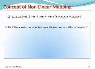
Concept of Non-LinearMapping
The 3-D input vector can be mapped into a 6-D space using the following mappings:
𝑋 (𝑥1 ,𝑥2 ,𝑥3)=𝑤1 𝑥1+𝑤1 𝑥1+𝑤1 𝑥1+𝑤4 𝑥1
2
+𝑤5 𝑥1 𝑥2+𝑤6 𝑥1 𝑥3+𝑏
Support Vector Machine
81.
81
Concept of Non-LinearMapping
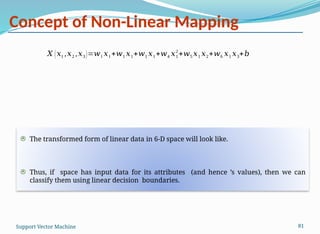
The transformed form of linear data in 6-D space will look like.
Thus, if space has input data for its attributes (and hence ’s values), then we can
classify them using linear decision boundaries.
𝑋 (𝑥1 ,𝑥2 ,𝑥3)=𝑤1 𝑥1+𝑤1 𝑥1+𝑤1 𝑥1+𝑤4 𝑥1
2
+𝑤5 𝑥1 𝑥2+𝑤6 𝑥1 𝑥3+𝑏
Support Vector Machine
82.
82
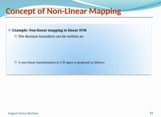
Concept of Non-LinearMapping
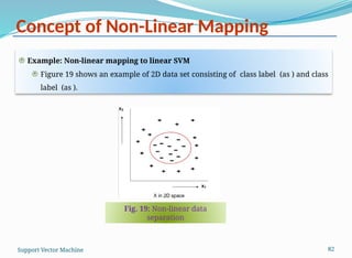
Example: Non-linear mapping to linear SVM
Figure 19 shows an example of 2D data set consisting of class label (as ) and class
label (as ).
Fig. 19: Non-linear data
separation
Support Vector Machine
83.
83
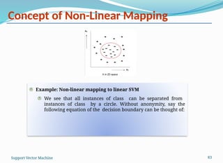
Concept of Non-LinearMapping
Example: Non-linear mapping to linear SVM
We see that all instances of class can be separated from
instances of class by a circle. Without anonymity, say the
following equation of the decision boundary can be thought of:
Support Vector Machine
84.
84
Concept of Non-LinearMapping
Example: Non-linear mapping to linear SVM
The decision boundary can be written as:
A non-linear transformation in 2-D space is proposed as follows:
Support Vector Machine
85.
85
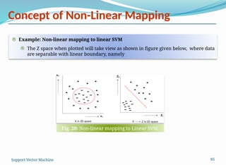
Concept of Non-LinearMapping
Example: Non-linear mapping to linear SVM
The Z space when plotted will take view as shown in figure given below, where data
are separable with linear boundary, namely
Fig. 20: Non-linear mapping to Linear SVM.
Support Vector Machine
86.
86
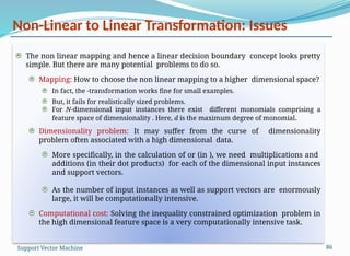
Non-Linear to LinearTransformation: Issues
The non linear mapping and hence a linear decision boundary concept looks pretty
simple. But there are many potential problems to do so.
Mapping: How to choose the non linear mapping to a higher dimensional space?
In fact, the -transformation works fine for small examples.
But, it fails for realistically sized problems.
For N-dimensional input instances there exist different monomials comprising a
feature space of dimensionality . Here, d is the maximum degree of monomial.
Dimensionality problem: It may suffer from the curse of dimensionality
problem often associated with a high dimensional data.
More specifically, in the calculation of or (in ), we need multiplications and
additions (in their dot products) for each of the dimensional input instances
and support vectors.
As the number of input instances as well as support vectors are enormously
large, it will be computationally intensive.
Computational cost: Solving the inequality constrained optimization problem in
the high dimensional feature space is a very computationally intensive task.
Support Vector Machine
87.
87
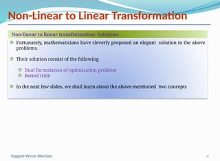
Non-Linear to LinearTransformation: Solution
Fortunately, mathematicians have cleverly proposed an elegant solution to the above
problems.
Their solution consist of the following:
Dual formulation of optimization problem
Kernel trick
In the next few lectures, we shall learn about the above-mentioned two concepts.
Support Vector Machine
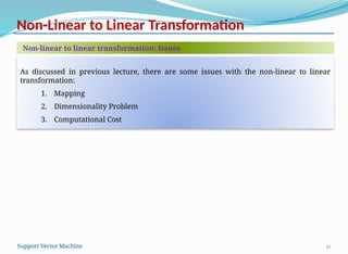
Non-Linear to LinearTransformation
89
As discussed in previous lecture, there are some issues with the non-linear to linear
transformation:
1. Mapping
2. Dimensionality Problem
3. Computational Cost
Non-linear to linear transformation: Issues
Support Vector Machine
90.
Non-Linear to LinearTransformation
90
Fortunately, mathematicians have cleverly proposed an elegant solution to the above
problems.
Their solution consist of the following
Dual formulation of optimization problem
Kernel trick
In the next few slides, we shall learn about the above-mentioned two concepts
Non-linear to linear transformation: Solutions
Support Vector Machine
Primal Form ofOptimization Problem
92
We have already learned the Lagrangian formulation to find the maximum margin
hyperplane for a linear SVM classifier.
Such a formulation is called primal form of the constraint optimization problem.
Primal form of the optimization problem is reproduced further
The primal form
Support Vector Machine
93.
Primal Form ofOptimization
93
The primal form of the above mentioned inequality constraint optimization problem
(according to Lagrange multiplier method) is given by
where, is called the Lagrangian multipliers
Here, is called the primal form of the Lagrange optimization problem
The primal form of the optimization problem
Support Vector Machine
94.
Dual Formulation ofOptimization Problem
94
The dual form of the same problem can be derived (from ) as follows:
Note that to minimize the optimization problem, we must take the derivative of with
respect to , and set them to zero.
The Dual form from the primal form
𝐿𝑝=
‖𝑊‖
2
2
−∑
𝑖=1
𝑛
𝜆𝑖 (𝑦𝑖 (𝑊 . 𝑥𝑖+𝑏)−1)
Support Vector Machine
95.
Dual Formulation ofOptimization Problem
95
From the above two equations, we get the Lagrangian as
The Dual form from the primal form
This form is called the Dual form of Lagrangian and distinguishably written as:
𝐿𝑝=
‖𝑊‖
2
2
−∑
𝑖=1
𝑛
𝜆𝑖 (𝑦𝑖 (𝑊 . 𝑥𝑖+𝑏)−1)
𝛿 𝐿𝑝
𝛿 𝑊
=0⇒ 𝑊 =∑
𝑖=1
𝑛
𝜆𝑖 𝑦𝑖 𝑥𝑖 ;
𝛿 𝐿𝑝
𝛿𝑏
=0 ⇒ ∑
𝑖=1
𝑛
𝜆𝑖 𝑦𝑖=0
Support Vector Machine
96.
Dual Form versusPrimal Form
96
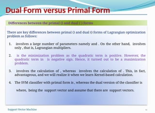
There are key differences between primal () and dual () forms of Lagrangian optimization
problem as follows:
1. involves a large number of parameters namely and . On the other hand, involves
only , that is, Lagrangian multipliers.
2. is the minimization problem as the quadratic term is positive. However, the
quadratic term in is negative sign. Hence, it turned out to be a maximization
problem.
3. involves the calculation of , whereas involves the calculation of . This, in fact,
advantageous, and we will realize it when we learn Kernel-based calculation.
4. The SVM classifier with primal form is , whereas the dual version of the classifier is
where, being the support vector and assume that there are support vectors.
Differences between the primal () and dual ( ) forms
Support Vector Machine
Dealing with Non-linearData
98
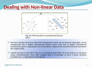
We have already learned an idea that training data which are not linearly separable, can be
transformed into a higher dimensional feature space such that in higher dimensional
transformed space a hyperplane can be decided to separate the transformed data and hence
the original data.
Clearly the data on the left in Fig. 21 is not linearly separable. Yet if we map it to a 3D space
using -transformation, then with mapped data it is possible to have a linear decision
boundary (i.e., a hyperplane in 3D space).
Fig. 21: SVM classifier in transformed feature
space
Support Vector Machine
99.
Dealing with Non-linearData
99
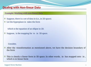
Suppose, there is a set of data in (i.e., in 2D space).
Let the hyperplane in takes the form
which is the equation of an ellipse in 2D.
Suppose, is the mapping for to in 3D space.
Consider,
After the -transformation as mentioned above, we have the decision boundary of
the form
This is clearly a linear form in 3D space. In other words, in has mapped onto in ,
which is in linear form
Example: Working with non-linear data
Support Vector Machine
100.
Dealing with Non-linearData
100
This means that data which are not linearly separable in 2D are separable in 3D. This
implies that the non-linear data can be classified by a linear SVM classifier.
The generalization of this formulation is provided next, which is key to kernel trick.
Conclusion: Linear SVM classifier is possible for classifying non-linear data
Support Vector Machine
Kernel Trick
102
Now, questionhere is how to choose φ, the mapping function X ⇒ Z , so that linear SVM
can be directly applied to?
A breakthrough solution to this problem comes in the form of a method as the kernel
trick.
The kernel trick is as follows.
We know that (.) dot product is often regarded as a measure of similarity between two
input vectors.
For example, if X and Y are two vectors, then
Here, similarity between X and Y is measured as cosine similarity.
If (i.e., ), then they are most similar, otherwise orthogonal, means dissimilar.
How to choose the mapping function φ?
Support Vector Machine
103.
Kernel Trick
103
Analogously, ifand are two tuples, then . is regarded as a measure of similarity
between and
Again, () and () are the transformed features of and , respectively in the transformed
space; thus, ().() is also should be regarded as the similarity measure between () and ()
in the transformed space.
This is an important revelation and is the basic idea behind the kernel trick.
Now, naturally question arises, if both measures the similarity, then what is the
correlation between them (i.e., . and ().()).
Let us try to find the answer to this question through an example.
How to choose the mapping function φ?
Support Vector Machine
104.
Kernel Trick
104
Without theloss of generality, let us consider a situation stated below:
Suppose, and are any two vectors in
Similarly,
and
are two transformed version of and in
Example: Correlation between . and ().()
Support Vector Machine
Kernel Trick
106
With referenceto the above example, we can conclude that are correlated to
In fact, the same can be proved, in general, for any feature vectors and their
transformed feature vectors. A formal proof is beyond the scope of this presentation.
More specifically, there is a correlation between dot products of original data and dot
products of transformed data.
Based on the above discussion, we can write the following implications:
Here, denotes a function more popularly called as Kernel function
Example: Correlation between . and ().()
Support Vector Machine
The Implication ofKernel Trick
109
This kernel function physically implies the similarity in the transformed space (i.e.,
non-linear similarity measure) using the original attribute
In other words, , the similarity function to compute a similarity of both whether data in
original attribute space or in transformed attribute space.
Significance of Kernel Trick
Support Vector Machine
110.
Kernel Trick andSVM
110
Implicit transformation: The first and foremost significance is that we do not require
any -transformation to the original input data at all! This is evident from the following
re-writing of our SVM classification problem.
Subject to,
Learning:
Classifier:
Formulation of SVM with Kernel trick
Support Vector Machine
111.
Kernel Trick andits Advantage
111
Computational efficiency:
Kernel trick allows an easy and efficient computability.
We know that in a SVM classifier, we need several and repeated round of computation
of dot products both in learning phase as well as in classification phase.
On other hand, using Kernel trick, we can do it once and with fewer dot products.
This is explained next.
Application of Kernel trick
Support Vector Machine
112.
Kernel Trick andits Advantage
112
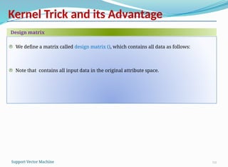
We define a matrix called design matrix (), which contains all data as follows:
Note that contains all input data in the original attribute space.
Design matrix
Support Vector Machine
113.
Kernel Trick andits Advantage
113
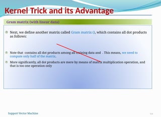
Next, we define another matrix called Gram matrix (), which contains all dot products
as follows:
Note that contains all dot products among all training data and . This means, we need to
compute only half of the matrix.
More significantly, all dot products are mere by means of matrix multiplication operation, and
that is too one operation only
Gram matrix (with linear data)
Support Vector Machine
114.
Kernel Trick andits Advantage
114
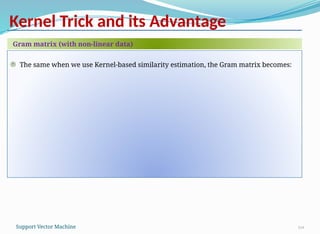
The same when we use Kernel-based similarity estimation, the Gram matrix becomes:
Gram matrix (with non-linear data)
Support Vector Machine
115.
SVM with KernelTrick
115
In nutshell, we have the following.
Instead of mapping our data viaand computing the dot products, we can accomplish
everything in one operation.
Classifier can be learnt and applied without explicitly computing .
Complexity of learning depends on (typically it is ), not on , the dimensionality of data
space.
All that is required is the kernel .
Next, we discuss the aspect of deciding kernel functions.
Summary of Kernel trick
Support Vector Machine
Kernel Functions
117
Before goingto learn the popular kernel functions adopted in SVM classification, we give
a precise and formal definition of kernel
Formal definition of Kernel function
A kernel function is a real valued function defined on , such that there is another
function a.
Symbolically, we write where .
Support Vector Machine
118.
Well Known KernelFunctions
118
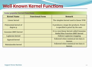
Some popular kernel functions
Kernel Name Functional Form Remark
Linear kernel The simplest kernel used in linear SVM
Polynomial kernel of
degree p
It produces a large dot products. Power
is specified a priori by the user.
Gaussian (RBF) kernel
It is a non-linear kernel called Gaussian
Radial Bias Function (RBF) kernel
Laplacian kernel Follows Laplacian mapping
Sigmoid kernel
Followed when statistical test data is
known
Mahalanobis kernel
Followed when statistical test data is
known
Support Vector Machine
119.
Kernel Functions: Example
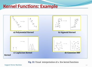
119
a)Polynomial Kernel b) Sigmoid Kernel
c) Laplacian Kernel d) Gaussian RBF
Kernel
Fig. 22: Visual interpretation of a few kernel functions
Support Vector Machine
Kernel Functions: Properties
121
Otherthan the standard kernel functions, we can define of our own kernels as well as
combining two or more kernels to another kernel.
If and are two kernels then,
are also valid Kernels.
Here,
Properties of kernel functions
Support Vector Machine
122.
Kernel Functions: Properties
122
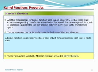
Anotherrequirement for kernel function used in non-linear SVM is that there must
exist a corresponding transformation such that the kernel function computed for a pair
of vectors is equivalent to the dot product between the vectors in the transformed
space.
This requirement can be formally stated in the form of Mercer’s theorem.
Mercer’s Theorem
A kernel function can be expressed as if and only if, for any function such that is finite
then
The kernels which satisfy the Mercer’s theorem are called Mercer kernels.
Support Vector Machine
123.
Kernel functions: Properties
123
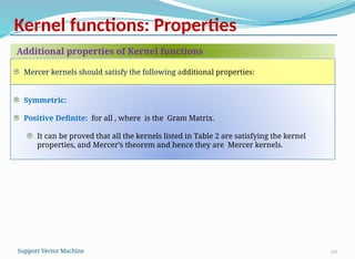
Symmetric:
PositiveDefinite: for all , where is the Gram Matrix.
It can be proved that all the kernels listed in Table 2 are satisfying the kernel
properties, and Mercer’s theorem and hence they are Mercer kernels.
Additional properties of Kernel functions
Mercer kernels should satisfy the following additional properties:
Support Vector Machine
Conclusions
125
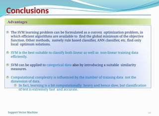
The SVM learningproblem can be formulated as a convex optimization problem, in
which efficient algorithms are available to find the global minimum of the objective
function. Other methods, namely rule based classifier, ANN classifier, etc. find only
local optimum solutions.
SVM is the best suitable to classify both linear as well as non-linear training data
efficiently.
SVM can be applied to categorical data also by introducing a suitable similarity
measures.
Computational complexity is influenced by the number of training data not the
dimension of data.
In fact, learning is a bit computationally heavy and hence slow, but classification
of test is extremely fast and accurate.
Advantages
Support Vector Machine
126.
REFERENCES
The detail materialrelated to this lecture can be found in
Data Mining: Concepts and Techniques, (3rd
Edn.), Jiawei Han, Micheline Kamber, Morgan Kaufmann,
2015.
Introduction to Data Mining, Pang-Ning Tan, Michael Steinbach, and Vipin Kumar, Addison-Wesley, 2014
Support Vector Machine 126
![Representation of MMH
23
In matrix form, a hyperplane can be represented as
where and and b is a real constant.
Here, W and b are parameters of the classifier model to be
learned given a training data set D
Equation of a hyperplane in matrix form
[
𝑥1
𝑥2
∙
∙
∙
𝑥𝑚
]
Support Vector Machine](https://image.slidesharecdn.com/08supportvectormachine-250215051023-a40894aa/85/Predictive-analytics-using-R-Programming-23-320.jpg)
![MMH for Linear SVM
29
We learnt,
The equation of the hyperplane
in matrix form is:
where and and b is a real
constant.
Thus, if we label all ’s are as
class label and all ’s are
class label , then we can
predict the class label for
any test data X as
RECAP: Equation of the hyperplane in matrix form
Fig. 8: Margin of the MMH
[
𝑥1
𝑥2
∙
∙
∙
𝑥𝑚
]
Support Vector Machine](https://image.slidesharecdn.com/08supportvectormachine-250215051023-a40894aa/85/Predictive-analytics-using-R-Programming-29-320.jpg)
![59
Illustration : Linear SVM
The parameter can be calculated for each support vector as follows
// for support vector
//using dot product
// for support vector
//using dot product
Averaging these values of and , we get .
W = [-6.64 -9.32]
x1 = [0.38 0.47]
x2 = [0.49 0.61]
Support Vector Machine](https://image.slidesharecdn.com/08supportvectormachine-250215051023-a40894aa/85/Predictive-analytics-using-R-Programming-59-320.jpg)


![[ML]-SVM2.ppt.pdf](https://cdn.slidesharecdn.com/ss_thumbnails/ml-svm2-230916145832-2580c8e3-thumbnail.jpg?width=640&height=640&fit=bounds)


![SVM[Support vector Machine] Machine learning](https://cdn.slidesharecdn.com/ss_thumbnails/svm-250403184638-1cd9afdb-thumbnail.jpg?width=640&height=640&fit=bounds)


![Attack surfaces and attack tress[inform]](https://cdn.slidesharecdn.com/ss_thumbnails/lecture03-260108015941-a4dee53b-thumbnail.jpg?width=640&height=640&fit=bounds)


