Predictive analytics using 'R' Programming 4

1. Classification: Naïve Bayes’ Classifier

2. Today’s discussion…
 Introduction to Classification
 Classification Techniques
 Supervised and unsupervised classifications
 Formal statement of supervised classification technique
 Bayesian Classifier
 Principle of Bayesian classifier
 Bayes’ theorem of probability
 Naïve Bayesian Classifier
 Addressing some issues with Naïve Bayesian Classifier
 Case study 2

3. 3
A Simple Quiz: Identify the objects

4. Introduction to Classification
4
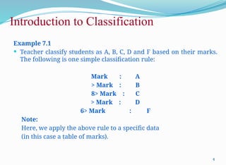
Example 7.1
 Teacher classify students as A, B, C, D and F based on their marks.
The following is one simple classification rule:
Mark : A
> Mark : B
8> Mark : C
> Mark : D
6> Mark : F
Note:
Here, we apply the above rule to a specific data
(in this case a table of marks).

5. Examples of Classification in Data Analytics
5
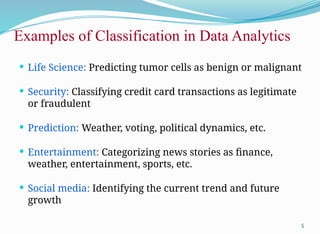
 Life Science: Predicting tumor cells as benign or malignant
 Security: Classifying credit card transactions as legitimate
or fraudulent
 Prediction: Weather, voting, political dynamics, etc.
 Entertainment: Categorizing news stories as finance,
weather, entertainment, sports, etc.
 Social media: Identifying the current trend and future
growth

6. Classification : Definition
6
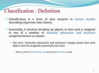
 Classification is a form of data analysis to extract models
describing important data classes.
 Essentially, it involves dividing up objects so that each is assigned
to one of a number of mutually exhaustive and exclusive
categories known as classes.
 The term “mutually exhaustive and exclusive” simply means that each
object must be assigned to precisely one class
 That is, never to more than one and never to no class at all.

7. Classification Techniques
7
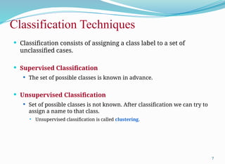
 Classification consists of assigning a class label to a set of
unclassified cases.
 Supervised Classification
 The set of possible classes is known in advance.
 Unsupervised Classification
 Set of possible classes is not known. After classification we can try to
assign a name to that class.
 Unsupervised classification is called clustering.

8. Supervised Classification
8

9. Unsupervised Classification
9

10. Supervised Classification Technique
10
 Given a collection of records (training set )
 Each record contains a set of attributes, one of the attributes is
the class.
 Find a model for class attribute as a function of the
values of other attributes.
 Goal: Previously unseen records should be assigned a
class as accurately as possible.
 Satisfy the property of “mutually exclusive and exhaustive”

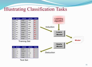
11. Illustrating Classification Tasks
11
Apply
Model
Induction
Deduction
Learn
Model
Model
Tid Attrib1 Attrib2 Attrib3 Class
1 Yes Large 125K No
2 No Medium 100K No
3 No Small 70K No
4 Yes Medium 120K No
5 No Large 95K Yes
6 No Medium 60K No
7 Yes Large 220K No
8 No Small 85K Yes
9 No Medium 75K No
10 No Small 90K Yes
10
Tid Attrib1 Attrib2 Attrib3 Class
11 No Small 55K ?
12 Yes Medium 80K ?
13 Yes Large 110K ?
14 No Small 95K ?
15 No Large 67K ?
10
Test Set
Learning
algorithm
Training Set

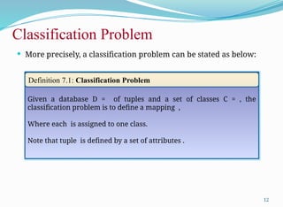
12. Classification Problem
12
 More precisely, a classification problem can be stated as below:
Given a database D = of tuples and a set of classes C = , the
classification problem is to define a mapping ,
Where each is assigned to one class.
Note that tuple is defined by a set of attributes .
Definition 7.1: Classification Problem

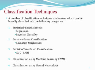
13. Classification Techniques
13
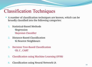
 A number of classification techniques are known, which can be
broadly classified into the following categories:
1. Statistical-Based Methods
•Regression
•Bayesian Classifier
•
2. Distance-Based Classification
•K-Nearest Neighbours
3. Decision Tree-Based Classification
•ID, C , CART
5. Classification using Machine Learning (SVM)
6. Classification using Neural Network (A

14. Classification Techniques
14
 A number of classification techniques are known, which can be
broadly classified into the following categories:
1. Statistical-Based Methods
•Regression
•Bayesian Classifier
•
2. Distance-Based Classification
•K-Nearest Neighbours
3. Decision Tree-Based Classification
•ID, C , CART
5. Classification using Machine Learning (SVM)
6. Classification using Neural Network (A

15. Bayesian Classifier
15

16. Bayesian Classifier
16
 Principle
 If it walks like a duck, quacks like a duck, then it is probably a duck

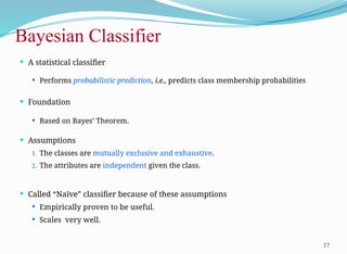
17.  A statistical classifier
 Performs probabilistic prediction, i.e., predicts class membership probabilities
 Foundation
 Based on Bayes’ Theorem.
 Assumptions
1. The classes are mutually exclusive and exhaustive.
2. The attributes are independent given the class.
 Called “Naïve” classifier because of these assumptions
 Empirically proven to be useful.
 Scales very well.
17
Bayesian Classifier

18. Example: Bayesian Classification
18
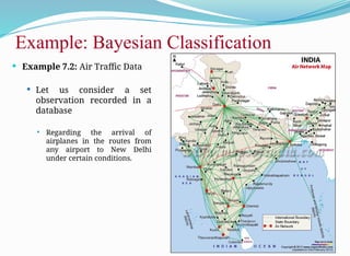
 Example 7.2: Air Traffic Data
 Let us consider a set
observation recorded in a
database
 Regarding the arrival of
airplanes in the routes from
any airport to New Delhi
under certain conditions.

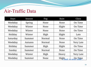
19. Air-Traffic Data
19
Days Season Fog Rain Class
Weekday Spring None None On Time
Weekday Winter None Slight On Time
Weekday Winter None None On Time
Holiday Winter High Slight Late
Saturday Summer Normal None On Time
Weekday Autumn Normal None Very Late
Holiday Summer High Slight On Time
Sunday Summer Normal None On Time
Weekday Winter High Heavy Very Late
Weekday Summer None Slight On Time
Cond. to next slide…

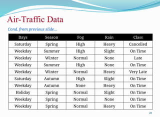
20. Air-Traffic Data
20
Days Season Fog Rain Class
Saturday Spring High Heavy Cancelled
Weekday Summer High Slight On Time
Weekday Winter Normal None Late
Weekday Summer High None On Time
Weekday Winter Normal Heavy Very Late
Saturday Autumn High Slight On Time
Weekday Autumn None Heavy On Time
Holiday Spring Normal Slight On Time
Weekday Spring Normal None On Time
Weekday Spring Normal Heavy On Time
Cond. from previous slide…

21. Air-Traffic Data
21
 In this database, there are four attributes
A = [ Day, Season, Fog, Rain]
with 20 tuples.
 The categories of classes are:
C= [On Time, Late, Very Late, Cancelled]
 Given this is the knowledge of data and classes, we are to find most
likely classification for any other unseen instance, for example:
 Classification technique eventually to map this tuple into an
accurate class.
Week
Day
Winter High None ???

22. Bayesian Classifier
22
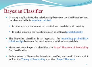
 In many applications, the relationship between the attributes set and
the class variable is non-deterministic.
 In other words, a test cannot be classified to a class label with certainty.
 In such a situation, the classification can be achieved probabilistically.
 The Bayesian classifier is an approach for modelling probabilistic
relationships between the attribute set and the class variable.
 More precisely, Bayesian classifier use Bayes’ Theorem of Probability
for classification.
 Before going to discuss the Bayesian classifier, we should have a quick
look at the Theory of Probability and then Bayes’ Theorem.

23. Bayes’ Theorem of Probability
23

24. Simple Probability
24
If there are n elementary events associated with a random experiment and m of n
of them are favorable to an event A, then the probability of happening or
occurrence of A is
Definition 7.2: Simple Probability

25. Simple Probability
25
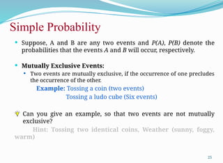
 Suppose, A and B are any two events and P(A), P(B) denote the
probabilities that the events A and B will occur, respectively.
 Mutually Exclusive Events:
 Two events are mutually exclusive, if the occurrence of one precludes
the occurrence of the other.
Example: Tossing a coin (two events)
Tossing a ludo cube (Six events)
Can you give an example, so that two events are not mutually
exclusive?
Hint: Tossing two identical coins, Weather (sunny, foggy,
warm)

26. Simple Probability
26
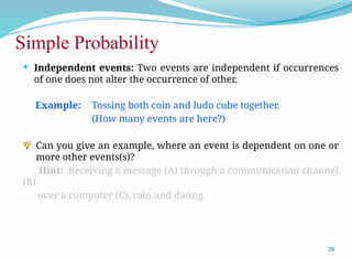
 Independent events: Two events are independent if occurrences
of one does not alter the occurrence of other.
Example: Tossing both coin and ludo cube together.
(How many events are here?)
Can you give an example, where an event is dependent on one or
more other events(s)?
Hint: Receiving a message (A) through a communication channel
(B)
over a computer (C), rain and dating.

27. Joint Probability
27
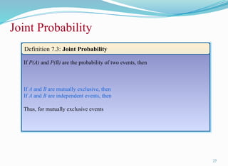
If P(A) and P(B) are the probability of two events, then
If A and B are mutually exclusive, then
If A and B are independent events, then
Thus, for mutually exclusive events
Definition 7.3: Joint Probability

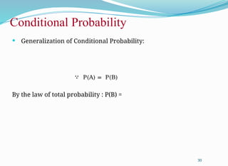
28. Conditional Probability
28
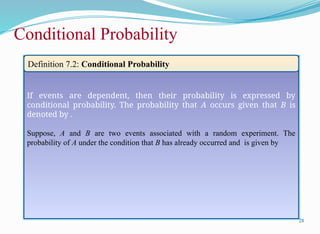
If events are dependent, then their probability is expressed by
conditional probability. The probability that A occurs given that B is
denoted by .
Suppose, A and B are two events associated with a random experiment. The
probability of A under the condition that B has already occurred and is given by
Definition 7.2: Conditional Probability

29. Conditional Probability
29
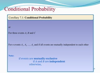
or
For three events A, B and C
For n events A1, A2, …, An and if all events are mutually independent to each other
Note:
if events are mutually exclusive
if A and B are independent
otherwise,
Corollary 7.1: Conditional Probability

30. Conditional Probability
30
 Generalization of Conditional Probability:
∵ P(A) = P(B)
By the law of total probability : P(B) =

31. Conditional Probability
31
In general,

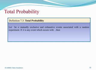
32. 32
Total Probability
CS 40003: Data Analytics 32
Let be n mutually exclusive and exhaustive events associated with a random
experiment. If A is any event which occurs with , then
Definition 7.3: Total Probability

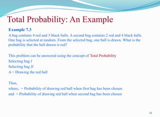
33. Example 7.3
A bag contains 4 red and 3 black balls. A second bag contains 2 red and 4 black balls.
One bag is selected at random. From the selected bag, one ball is drawn. What is the
probability that the ball drawn is red?
This problem can be answered using the concept of Total Probability
Selecting bag I
Selecting bag II
A = Drawing the red ball
Thus,
where, = Probability of drawing red ball when first bag has been chosen
and = Probability of drawing red ball when second bag has been chosen
33
Total Probability: An Example

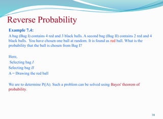
34. Example 7.4:
A bag (Bag I) contains 4 red and 3 black balls. A second bag (Bag II) contains 2 red and 4
black balls. You have chosen one ball at random. It is found as red ball. What is the
probability that the ball is chosen from Bag I?
Here,
Selecting bag I
Selecting bag II
A = Drawing the red ball
We are to determine P(|A). Such a problem can be solved using Bayes' theorem of
probability.
34
Reverse Probability

35. Bayes’ Theorem
35
Let be n mutually exclusive and exhaustive events associated with a random
experiment. If A is any event which occurs with , then
Theorem 7.4: Bayes’ Theorem

36. Prior and Posterior Probabilities
36
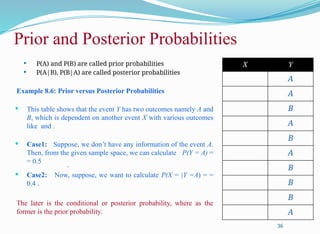
 P(A) and P(B) are called prior probabilities
 P(A|B), P(B|A) are called posterior probabilities
Example 8.6: Prior versus Posterior Probabilities
 This table shows that the event Y has two outcomes namely A and
B, which is dependent on another event X with various outcomes
like and .
 Case1: Suppose, we don’t have any information of the event A.
Then, from the given sample space, we can calculate P(Y = A) =
= 0.5
•
 Case2: Now, suppose, we want to calculate P(X = |Y =A) = =
0.4 .
The later is the conditional or posterior probability, where as the
former is the prior probability.
X Y
A
A
B
A
B
A
B
B
B
A

37. Naïve Bayesian Classifier
37
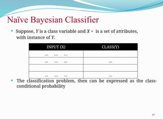
 Suppose, Y is a class variable and X = is a set of attributes,
with instance of Y.
 The classification problem, then can be expressed as the class-
conditional probability
INPUT (X) CLASS(Y)
… … …
… … … …
… … … …

38. Naïve Bayesian Classifier
38
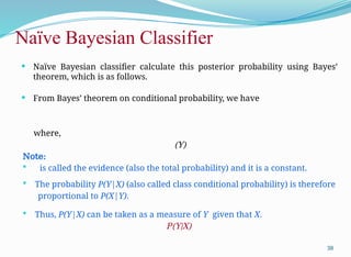
 Naïve Bayesian classifier calculate this posterior probability using Bayes’
theorem, which is as follows.
 From Bayes’ theorem on conditional probability, we have
where,
(Y)
Note:
 is called the evidence (also the total probability) and it is a constant.
 The probability P(Y|X) (also called class conditional probability) is therefore
proportional to P(X|Y).
 Thus, P(Y|X) can be taken as a measure of Y given that X.
P(Y|X)

39. Naïve Bayesian Classifier
39
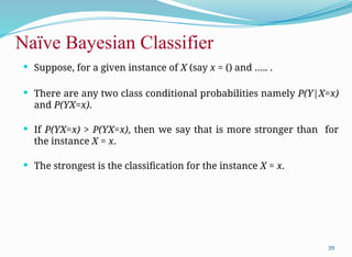
 Suppose, for a given instance of X (say x = () and ….. .
 There are any two class conditional probabilities namely P(Y|X=x)
and P(YX=x).
 If P(YX=x) > P(YX=x), then we say that is more stronger than for
the instance X = x.
 The strongest is the classification for the instance X = x.

40. Naïve Bayesian Classifier
40
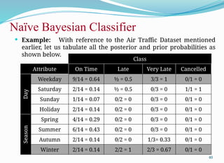
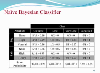
 Example: With reference to the Air Traffic Dataset mentioned
earlier, let us tabulate all the posterior and prior probabilities as
shown below.
Class
Attribute On Time Late Very Late Cancelled
Day
Weekday 9/14 = 0.64 ½ = 0.5 3/3 = 1 0/1 = 0
Saturday 2/14 = 0.14 ½ = 0.5 0/3 = 0 1/1 = 1
Sunday 1/14 = 0.07 0/2 = 0 0/3 = 0 0/1 = 0
Holiday 2/14 = 0.14 0/2 = 0 0/3 = 0 0/1 = 0
Season
Spring 4/14 = 0.29 0/2 = 0 0/3 = 0 0/1 = 0
Summer 6/14 = 0.43 0/2 = 0 0/3 = 0 0/1 = 0
Autumn 2/14 = 0.14 0/2 = 0 1/3= 0.33 0/1 = 0
Winter 2/14 = 0.14 2/2 = 1 2/3 = 0.67 0/1 = 0

41. Naïve Bayesian Classifier
41
Class
Attribute On Time Late Very Late Cancelled
Fog
None 5/14 = 0.36 0/2 = 0 0/3 = 0 0/1 = 0
High 4/14 = 0.29 1/2 = 0.5 1/3 = 0.33 1/1 = 1
Normal 5/14 = 0.36 1/2 = 0.5 2/3 = 0.67 0/1 = 0
Rain
None 5/14 = 0.36 1/2 = 0.5 1/3 = 0.33 0/1 = 0
Slight 8/14 = 0.57 0/2 = 0 0/3 = 0 0/1 = 0
Heavy 1/14 = 0.07 1/2 = 0.5 2/3 = 0.67 1/1 = 1
Prior
Probability
14/20 = 0.70 2/20 = 0.10 3/20 = 0.15 1/20 = 0.05

42. Naïve Bayesian Classifier
42
Instance:
Case1: Class = On Time : 0.70 × 0.64 × 0.14 × 0.29 × 0.07 = 0.0013
Case2: Class = Late : 0.10 × 0.50 × 1.0 × 0.50 × 0.50 = 0.0125
Case3: Class = Very Late : 0.15 × 1.0 × 0.67 × 0.33 × 0.67 = 0.0222
Case4: Class = Cancelled : 0.05 × 0.0 × 0.0 × 1.0 × 1.0 = 0.0000
Case3 is the strongest; Hence correct classification is Very Late
Week
Day
Winter High Heavy ???

43. Naïve Bayesian Classifier
43
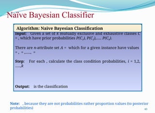
Note: , because they are not probabilities rather proportion values (to posterior
probabilities)
Input: Given a set of k mutually exclusive and exhaustive classes C
= , which have prior probabilities P(C1), P(C2),….. P(Ck).
There are n-attribute set A = which for a given instance have values
= , = ,….., =
Step: For each , calculate the class condition probabilities, i = 1,2,
…..,k
Output: is the classification
Algorithm: Naïve Bayesian Classification

44. Naïve Bayesian Classifier
44
Pros and Cons
 The Naïve Bayes’ approach is a very popular one, which often
works well.
 However, it has a number of potential problems
 It relies on all attributes being categorical.
 If the data is less, then it estimates poorly.

45. Naïve Bayesian Classifier
45
Approaches to overcome the limitations in Naïve Bayesian
Classification
 Estimating the posterior probabilities for continuous attributes
 In real life situation, all attributes are not necessarily be categorical,
In fact, there is a mix of both categorical and continuous attributes.
 There are two approaches to deal with continuous attributes in
Bayesian classifier.
Approach 1:
We can discretize each continuous attributes and then replace the
continuous values with its corresponding discrete intervals.

46. Naïve Bayesian Classifier
46
 Estimating the posterior probabilities for continuous
attributes
Approach 2:
We can assume a certain form of probability distribution for the
continuous variable and estimate the parameters of the distribution
using the training data. A Gaussian distribution is usually chosen to
represent the posterior probabilities for continuous attributes. A
general form of Gaussian distribution will look like
where, denote mean and variance, respectively.

47. Naïve Bayesian Classifier
47
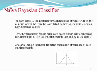
For each class Ci, the posterior probabilities for attribute Aj (it is the
numeric attribute) can be calculated following Gaussian normal
distribution as follows.
Here, the parameter can be calculated based on the sample mean of
attribute values of for the training records that belong to the class .
Similarly, can be estimated from the calculation of variance of such
training records.

48. Naïve Bayesian Classifier
48
 The M-estimation is to deal with the potential problem of
Naïve Bayesian Classifier when training data size is too poor.
 If the posterior probability for one of the attribute is zero, then
the overall class-conditional probability for the class vanishes.
 In other words, if training data do not cover many of the attribute
values, then we may not be able to classify some of the test
records.
 This problem can be addressed by using the M-estimate
approach.

49. M-estimate Approach
49
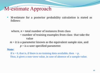
 M-estimate for a posterior probability calculation is stated as
follows:
where, n = total number of instances from class
= number of training examples from class that take the
value
m = it is a parameter known as the equivalent sample size, and
p = is a user specified parameter.
Note:
If n = 0, that is, if there is no training data available, then = p,
Thus, it gives a non=zero value, in case of absence of a sample value.

50. Case Study - 1
50
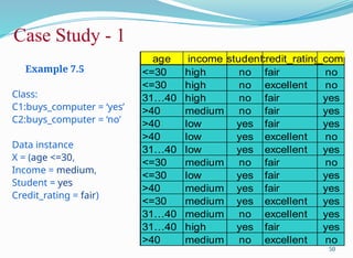
Example 7.5
age income student
credit_rating
buys_compu
<=30 high no fair no
<=30 high no excellent no
31…40 high no fair yes
>40 medium no fair yes
>40 low yes fair yes
>40 low yes excellent no
31…40 low yes excellent yes
<=30 medium no fair no
<=30 low yes fair yes
>40 medium yes fair yes
<=30 medium yes excellent yes
31…40 medium no excellent yes
31…40 high yes fair yes
>40 medium no excellent no
Class:
C1:buys_computer = ‘yes’
C2:buys_computer = ‘no’
Data instance
X = (age <=30,
Income = medium,
Student = yes
Credit_rating = fair)

51. Solution to Case Study -1
51
 P(Ci): P(buys_computer = “yes”) = 9/14 = 0.643
P(buys_computer = “no”) = 5/14= 0.357
 Compute P(X|Ci) for each class
P(age = “<=30” | buys_computer = “yes”) = 2/9 = 0.222
P(age = “<= 30” | buys_computer = “no”) = 3/5 = 0.6
P(income = “medium” | buys_computer = “yes”) = 4/9 = 0.444
P(income = “medium” | buys_computer = “no”) = 2/5 = 0.4
P(student = “yes” | buys_computer = “yes) = 6/9 = 0.667
P(student = “yes” | buys_computer = “no”) = 1/5 = 0.2
P(credit_rating = “fair” | buys_computer = “yes”) = 6/9 = 0.667
P(credit_rating = “fair” | buys_computer = “no”) = 2/5 = 0.4
 X = (age <= 30 , income = medium, student = yes, credit_rating = fair)
P(X|Ci) : P(X|buys_computer = “yes”) = 0.222 × 0.444 × 0.667 × 0.667 = 0.044
P(X|buys_computer = “no”) = 0.6 × 0.4 × 0.2 × 0.4 = 0.019
P(X|Ci)*P(Ci) : P(X|buys_computer = “yes”) * P(buys_computer = “yes”) = 0.028
P(X|buys_computer = “no”) * P(buys_computer = “no”) = 0.007
Therefore, X belongs to class (“buys_computer = yes”)

52. Case Study - 2
52
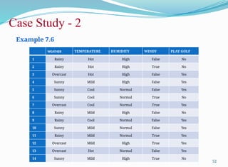
Example 7.6
WEATHER TEMPERATURE HUMIDITY WINDY PLAY GOLF
1 Rainy Hot High False No
2 Rainy Hot High True No
3 Overcast Hot High False Yes
4 Sunny Mild High False Yes
5 Sunny Cool Normal False Yes
6 Sunny Cool Normal True No
7 Overcast Cool Normal True Yes
8 Rainy Mild High False No
9 Rainy Cool Normal False Yes
10 Sunny Mild Normal False Yes
11 Rainy Mild Normal True Yes
12 Overcast Mild High True Yes
13 Overcast Hot Normal False Yes
14 Sunny Mild High True No

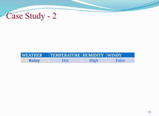
53. Case Study - 2
53
WEATHER TEMPERATURE HUMIDITY WINDY
Rainy Hot High False

54. Reference
54
 The detail material related to this lecture can be found in
Data Mining: Concepts and Techniques, (3rd
Edn.), Jiawei Han, Micheline Kamber,
Morgan Kaufmann, 2015.
Introduction to Data Mining, Pang-Ning Tan, Michael Steinbach, and Vipin Kumar,
Addison-Wesley, 2014