good book

1. INES-Ruhengeri
Faculty of Health
Sciences
Department of
Pharmacy
PROBABILITY
DISTRIBUTION
1

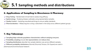
2. CONTENT
1. Basic Probability and Random Variables
2. Random Variables and Distributions
3. Common Probability Distributions
4. Joint Distributions and Covariance
5. Sampling and Estimation
6. Hypothesis Testing
2

3. 1. Basic Probability and Random
Variables
1.1 Counting arguments, permutations, and
combinations
1.2 Postulates and rules of probability
1.3 Conditional probability
3

4. 1.1 Counting arguments, permutations, and
combinations
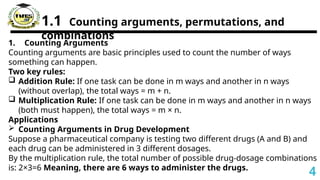
1. Counting Arguments
Counting arguments are basic principles used to count the number of ways
something can happen.
Two key rules:
 Addition Rule: If one task can be done in m ways and another in n ways
(without overlap), the total ways = m + n.
 Multiplication Rule: If one task can be done in m ways and another in n ways
(both must happen), the total ways = m × n.
Applications
 Counting Arguments in Drug Development
Suppose a pharmaceutical company is testing two different drugs (A and B) and
each drug can be administered in 3 different dosages.
By the multiplication rule, the total number of possible drug-dosage combinations
is: 2×3=6 Meaning, there are 6 ways to administer the drugs.
4

5. 1.1 Counting arguments, permutations, and
combinations
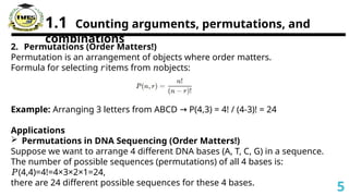
2. Permutations (Order Matters!)
Permutation is an arrangement of objects where order matters.
Formula for selecting items from objects:
𝑟 𝑛
Example: Arranging 3 letters from ABCD P(4,3) = 4! / (4-3)! = 24
→
Applications
 Permutations in DNA Sequencing (Order Matters!)
Suppose we want to arrange 4 different DNA bases (A, T, C, G) in a sequence.
The number of possible sequences (permutations) of all 4 bases is:
𝑃(4,4)=4!=4×3×2×1=24,
there are 24 different possible sequences for these 4 bases.
5

6. 1.1 Counting arguments, permutations, and
combinations
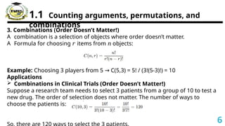
3. Combinations (Order Doesn’t Matter!)
A combination is a selection of objects where order doesn’t matter.
A Formula for choosing items from objects:
𝑟 𝑛
Example: Choosing 3 players from 5 C(5,3) = 5! / (3!(5-3)!) = 10
→
Applications
 Combinations in Clinical Trials (Order Doesn’t Matter!)
Suppose a research team needs to select 3 patients from a group of 10 to test a
new drug. The order of selection does not matter. The number of ways to
choose the patients is:
6

7. 1.1 Counting arguments, permutations, and
combinations
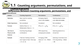
Differences Between Counting arguments, permutations, and
combinations
7

8. 1.2 Postulates and rules of probability
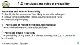
Postulates and Rules of Probability
Probability is the measure of how likely an event is to happen.
It follows certain postulates (basic assumptions) and rules
(mathematical principles).
1. Postulates of Probability (Basic Assumptions)
These are the three fundamental postulates:
 Postulate 1: Non-Negativity
The probability of any event is always non-negative (i.e., it cannot be
𝐴
less than 0).
Mathematically: ( ) 0
𝑃 𝐴 ≥ 8

9. 1.2 Postulates and rules of probability
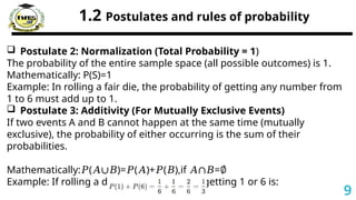
 Postulate 2: Normalization (Total Probability = 1)
The probability of the entire sample space (all possible outcomes) is 1.
Mathematically: P(S)=1
Example: In rolling a fair die, the probability of getting any number from
1 to 6 must add up to 1.
 Postulate 3: Additivity (For Mutually Exclusive Events)
If two events A and B cannot happen at the same time (mutually
exclusive), the probability of either occurring is the sum of their
probabilities.
Mathematically: ( )= ( )+ ( ),if =
𝑃 𝐴∪𝐵 𝑃 𝐴 𝑃 𝐵 𝐴∩𝐵 ∅
Example: If rolling a die, the probability of getting 1 or 6 is:
9

10. 1.2 Postulates and rules of probability
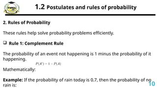
2. Rules of Probability
These rules help solve probability problems efficiently.
 Rule 1: Complement Rule
The probability of an event not happening is 1 minus the probability of it
happening.
Mathematically:
Example: If the probability of rain today is 0.7, then the probability of no
rain is: 10

11. 1.2 Postulates and rules of probability
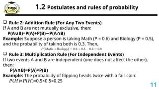
 Rule 2: Addition Rule (For Any Two Events)
If A and B are not mutually exclusive, then:
P(A B)=P(A)+P(B) P(A B)
∪ − ∩
Example: Suppose a person is taking Math (P = 0.6) and Biology (P = 0.5),
and the probability of taking both is 0.3. Then,
 Rule 3: Multiplication Rule (For Independent Events)
If two events A and B are independent (one does not affect the other),
then:
P(A B)=P(A)×P(B)
∩
Example: The probability of flipping heads twice with a fair coin:
𝑃( )× ( )=0.5×0.5=0.25
𝐻 𝑃 𝐻
11

12. 1.2 Postulates and rules of probability
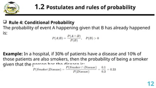
 Rule 4: Conditional Probability
The probability of event A happening given that B has already happened
is:
Example: In a hospital, if 30% of patients have a disease and 10% of
those patients are also smokers, then the probability of being a smoker
given that the person has the disease is:
12

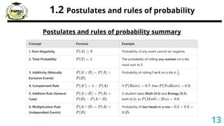
13. 1.2 Postulates and rules of probability
Postulates and rules of probability summary
13

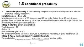
14. 1.3 Conditional probability
 Conditional probability is about finding the probability of an event given that another
event has already happened.
Simple Example – Real Life
Imagine you are in a class of 50 students, and 20 are girls. Out of these 20 girls, 8 wear
glasses. Now, suppose we already know that a randomly chosen student is a girl. What’s the
probability that this girl wears glasses?
🔹 Step 1: Identify Given Information
Total students = 50
Girls = 20
Girls who wear glasses = 8
We are given that the student is a girl, so our sample is now only 20 girls, not the full 50.
🔹 Step 2: Apply the Conditional Probability Formula
The probability that a student wears glasses given that she is a girl is:
14

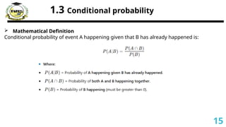
15. 1.3 Conditional probability
 Mathematical Definition
Conditional probability of event A happening given that B has already happened is:
15

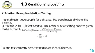
16. 1.3 Conditional probability
 Another Example – Medical Testing
hospital tests 1,000 people for a disease: 100 people actually have the
disease.
Out of these 100, 90 test positive. The probability of testing positive given
that a person has the disease is:
So, the test correctly detects the disease in 90% of cases.
16

17. 2. Random Variables and
Distributions
2.1 Discrete and continuous random variables
2.2 Probability distribution functions
2.3 Expectation, mean, variance, and moments of random variabl
2.4. Moment generating functions
17

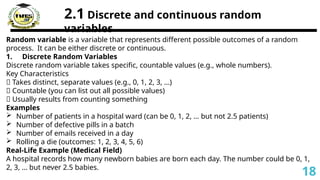
18. 2.1 Discrete and continuous random
variables
Random variable is a variable that represents different possible outcomes of a random
process. It can be either discrete or continuous.
1. Discrete Random Variables
Discrete random variable takes specific, countable values (e.g., whole numbers).
Key Characteristics
✅ Takes distinct, separate values (e.g., 0, 1, 2, 3, …)
✅ Countable (you can list out all possible values)
✅ Usually results from counting something
Examples
 Number of patients in a hospital ward (can be 0, 1, 2, … but not 2.5 patients)
 Number of defective pills in a batch
 Number of emails received in a day
 Rolling a die (outcomes: 1, 2, 3, 4, 5, 6)
Real-Life Example (Medical Field)
A hospital records how many newborn babies are born each day. The number could be 0, 1,
2, 3, … but never 2.5 babies.
18

19. 2.1 Discrete and continuous random
variables
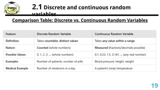
Comparison Table: Discrete vs. Continuous Random Variables
19

20. 2.1 Discrete and continuous random
variables
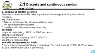
2. Continuous Random Variables
Continuous random variable takes any value within a range (including decimals and
fractions).
Key Characteristics
✅ Takes an infinite number of values within a range
✅ Not countable but measurable
✅ Usually results from measuring something
Examples
Height of patients (e.g., 170.2 cm, 170.25 cm, etc.)
Blood pressure levels
Temperature of a body (e.g., 36.5°C, 36.55°C)
Weight of a medicine dose
Real-Life Example (Medical Field)
A nurse measures a patient's body temperature. The result could be 37.0°C, 37.2°C, or even
37.23°C, meaning the value is continuous.
20

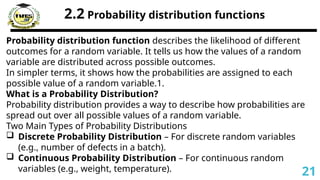
21. 2.2 Probability distribution functions
Probability distribution function describes the likelihood of different
outcomes for a random variable. It tells us how the values of a random
variable are distributed across possible outcomes.
In simpler terms, it shows how the probabilities are assigned to each
possible value of a random variable.1.
What is a Probability Distribution?
Probability distribution provides a way to describe how probabilities are
spread out over all possible values of a random variable.
Two Main Types of Probability Distributions
 Discrete Probability Distribution – For discrete random variables
(e.g., number of defects in a batch).
 Continuous Probability Distribution – For continuous random
variables (e.g., weight, temperature). 21

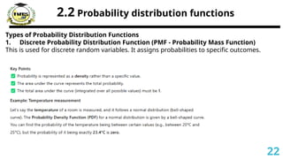
22. 2.2 Probability distribution functions
Types of Probability Distribution Functions
1. Discrete Probability Distribution Function (PMF - Probability Mass Function)
This is used for discrete random variables. It assigns probabilities to specific outcomes.
22

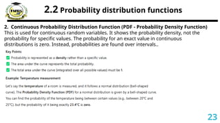
23. 2.2 Probability distribution functions
2. Continuous Probability Distribution Function (PDF - Probability Density Function)
This is used for continuous random variables. It shows the probability density, not the
probability for specific values. The probability for an exact value in continuous
distributions is zero. Instead, probabilities are found over intervals..
23

24. 2.2 Probability distribution functions
2. Continuous Probability Distribution Function (PDF - Probability Density Function)
This is used for continuous random variables. It shows the probability density, not the
probability for specific values. The probability for an exact value in continuous
distributions is zero. Instead, probabilities are found over intervals..
24

25. 2.2 Probability distribution functions
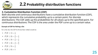
3. Cumulative Distribution Function (CDF)
Both discrete and continuous distributions have a cumulative distribution function (CDF),
which represents the cumulative probability up to a certain point. For discrete
distributions: The CDF adds up the probabilities for all values up to the specified point. For
continuous distributions: The CDF is the area under the PDF curve up to a certain value.
25

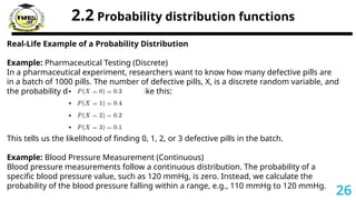
26. 2.2 Probability distribution functions
Real-Life Example of a Probability Distribution
Example: Pharmaceutical Testing (Discrete)
In a pharmaceutical experiment, researchers want to know how many defective pills are
in a batch of 1000 pills. The number of defective pills, X, is a discrete random variable, and
the probability distribution could be like this:
This tells us the likelihood of finding 0, 1, 2, or 3 defective pills in the batch.
Example: Blood Pressure Measurement (Continuous)
Blood pressure measurements follow a continuous distribution. The probability of a
specific blood pressure value, such as 120 mmHg, is zero. Instead, we calculate the
probability of the blood pressure falling within a range, e.g., 110 mmHg to 120 mmHg.
26

27. 2.2 Probability distribution functions
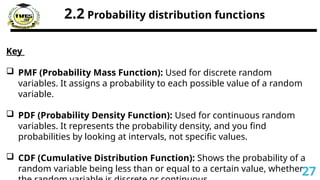
Key
 PMF (Probability Mass Function): Used for discrete random
variables. It assigns a probability to each possible value of a random
variable.
 PDF (Probability Density Function): Used for continuous random
variables. It represents the probability density, and you find
probabilities by looking at intervals, not specific values.
 CDF (Cumulative Distribution Function): Shows the probability of a
random variable being less than or equal to a certain value, whether27

28. 2.3 Expectation, mean, variance, and moments of
random variables
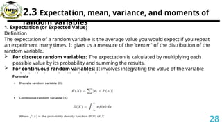
1. Expectation (or Expected Value)
Definition
The expectation of a random variable is the average value you would expect if you repeat
an experiment many times. It gives us a measure of the "center" of the distribution of the
random variable.
 For discrete random variables: The expectation is calculated by multiplying each
possible value by its probability and summing the results.
 For continuous random variables: It involves integrating the value of the variable
multiplied by its probability density function.
28

29. 2.3 Expectation, mean, variance, and moments of
random variables
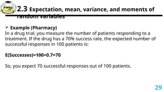
 Example (Pharmacy)
In a drug trial, you measure the number of patients responding to a
treatment. If the drug has a 70% success rate, the expected number of
successful responses in 100 patients is:
E(Successes)=100×0.7=70
So, you expect 70 successful responses out of 100 patients.
29

30. 2.3 Expectation, mean, variance, and moments of
random variables
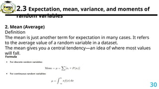
2. Mean (Average)
Definition
The mean is just another term for expectation in many cases. It refers
to the average value of a random variable in a dataset.
The mean gives you a central tendency—an idea of where most values
will fall.
30

31. 2.3 Expectation, mean, variance, and moments of
random variables
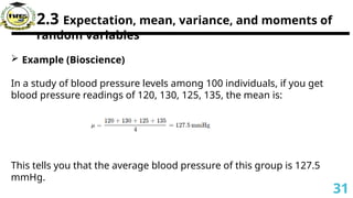
 Example (Bioscience)
In a study of blood pressure levels among 100 individuals, if you get
blood pressure readings of 120, 130, 125, 135, the mean is:
This tells you that the average blood pressure of this group is 127.5
mmHg.
31

32. 2.3 Expectation, mean, variance, and moments of
random variables
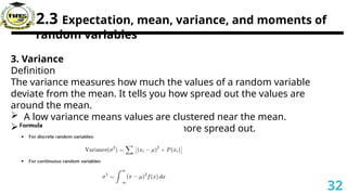
3. Variance
Definition
The variance measures how much the values of a random variable
deviate from the mean. It tells you how spread out the values are
around the mean.
 A low variance means values are clustered near the mean.
 A high variance means values are more spread out.
32

33. 2.3 Expectation, mean, variance, and moments of
random variables
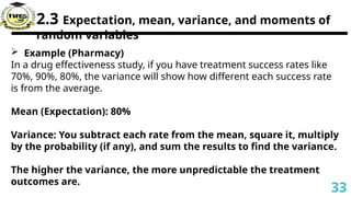
 Example (Pharmacy)
In a drug effectiveness study, if you have treatment success rates like
70%, 90%, 80%, the variance will show how different each success rate
is from the average.
Mean (Expectation): 80%
Variance: You subtract each rate from the mean, square it, multiply
by the probability (if any), and sum the results to find the variance.
The higher the variance, the more unpredictable the treatment
outcomes are.
33

34. 2.3 Expectation, mean, variance, and moments of
random variables
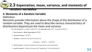
4. Moments of a Random Variable
Definition
Moments provide information about the shape of the distribution of a
random variable. They are used to describe various characteristics of
distributions beyond just the mean and variance.
34

35. 2.3 Expectation, mean, variance, and moments of
random variables
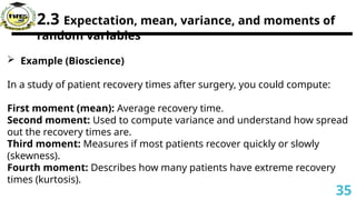
 Example (Bioscience)
In a study of patient recovery times after surgery, you could compute:
First moment (mean): Average recovery time.
Second moment: Used to compute variance and understand how spread
out the recovery times are.
Third moment: Measures if most patients recover quickly or slowly
(skewness).
Fourth moment: Describes how many patients have extreme recovery
times (kurtosis).
35

36. 2.3 Expectation, mean, variance, and moments of
random variables
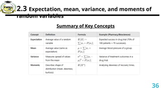
Summary of Key Concepts
36

37. 2.4 Moment generating functions
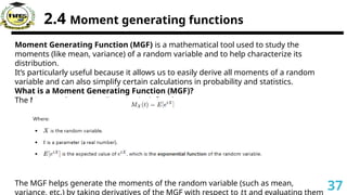
Moment Generating Function (MGF) is a mathematical tool used to study the
moments (like mean, variance) of a random variable and to help characterize its
distribution.
It’s particularly useful because it allows us to easily derive all moments of a random
variable and can also simplify certain calculations in probability and statistics.
What is a Moment Generating Function (MGF)?
The Moment Generating Function is defined as:
The MGF helps generate the moments of the random variable (such as mean,
variance, etc.) by taking derivatives of the MGF with respect to t and evaluating them
𝑡
37

38. 2.4 Moment generating functions
Why is the Moment Generating Function Useful?
 Generating Moments: The MGF can be used to find all the moments (mean,
variance, skewness, etc.) of a random variable.
 Simplification: MGFs can simplify certain calculations, especially when dealing
with sums of independent random variables.
 Characterizing Distributions: The MGF can uniquely identify a probability
distribution for a random variable, provided it exists.
38

39. 2.4 Moment generating functions
How to Use the MGF?
39

40. 2.4 Moment generating functions
Examples in Biosciences and Pharmacy
Example 1: Exponential Distribution (Pharmacy)
Let’s consider a pharmaceutical experiment where the time between successive
events (e.g., failure of a drug or time until a patient exhibits symptoms) follows an
exponential distribution.
40

41. 2.4 Moment generating functions
Example 2: Normal Distribution (Biosciences)
Now, let’s look at a normal distribution, which is often used to model biological
variables such as blood pressure, weight, and height.
So, you can see how the MGF provides quick access to both the mean and variance.
41

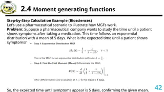
42. 2.4 Moment generating functions
Step-by-Step Calculation Example (Biosciences)
Let’s use a pharmaceutical scenario to illustrate how MGFs work.
Problem: Suppose a pharmaceutical company wants to study the time until a patient
shows symptoms after taking a medication. This time follows an exponential
distribution with a mean of 5 days. What is the expected time until a patient shows
symptoms?
So, the expected time until symptoms appear is 5 days, confirming the given mean. 42

43. 2.4 Moment generating functions
Step-by-Step Calculation Example (Biosciences)
Let’s use a pharmaceutical scenario to illustrate how MGFs work.
Problem: Suppose a pharmaceutical company wants to study the time until a patient
shows symptoms after taking a medication. This time follows an exponential
distribution with a mean of 5 days. What is the expected time until a patient shows
symptoms?
So, the expected time until symptoms appear is 5 days, confirming the given mean. 43

44. 3. Common Probability Distributions
3.1 Binomial, Poisson, and Geometric distributions
3.2 Normal, Uniform, and Gamma Beta distributions
3.3 Chi-square and F-distributions
44

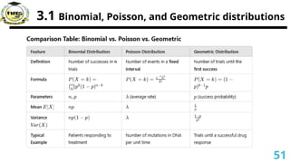
45. 3.1 Binomial, Poisson, and Geometric distributions
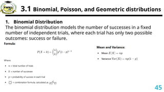
1. Binomial Distribution
The binomial distribution models the number of successes in a fixed
number of independent trials, where each trial has only two possible
outcomes: success or failure.
45

46. 3.1 Binomial, Poisson, and Geometric distributions
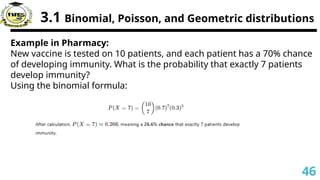
Example in Pharmacy:
New vaccine is tested on 10 patients, and each patient has a 70% chance
of developing immunity. What is the probability that exactly 7 patients
develop immunity?
Using the binomial formula:
46

47. 3.1 Binomial, Poisson, and Geometric distributions
2. Poisson Distribution
The Poisson distribution models the number of times an event occurs in
a fixed interval of time or space, given that events occur randomly and
independently at a constant rate.
47

48. 3.1 Binomial, Poisson, and Geometric distributions
Example in Biosciences:
Suppose a hospital receives 4 emergency cases per hour on average.
What is the probability that exactly 6 cases arrive in the next hour?
Using the Poisson formula:
48

49. 3.1 Binomial, Poisson, and Geometric distributions
3. Geometric Distribution
The geometric distribution models the number of trials needed until the
first success occurs. It is used when trials are repeated independently
with a constant probability of success.
49

50. 3.1 Binomial, Poisson, and Geometric distributions
Example in Pharmacy:
Pharmacist is testing a new drug on patients. The probability of the drug
successfully curing an infection in a single patient is 20% (p=0.2). What is
the probability that the first success occurs on the 3rd patient?
Using the geometric formula:
50

51. 3.1 Binomial, Poisson, and Geometric distributions
51

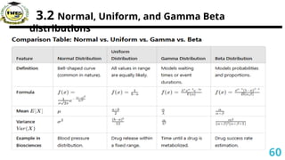
52. 3.2 Normal, Uniform, and Gamma Beta
distributions
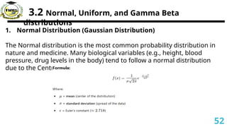
1. Normal Distribution (Gaussian Distribution)
The Normal distribution is the most common probability distribution in
nature and medicine. Many biological variables (e.g., height, blood
pressure, drug levels in the body) tend to follow a normal distribution
due to the Central Limit Theorem.
52

53. 3.2 Normal, Uniform, and Gamma Beta
distributions
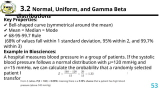
Key Properties:
✔ Bell-shaped curve (symmetrical around the mean)
✔ Mean = Median = Mode
✔ 68-95-99.7 Rule
(68% of values fall within 1 standard deviation, 95% within 2, and 99.7%
within 3)
Example in Biosciences:
A hospital measures blood pressure in a group of patients. If the systolic
blood pressure follows a normal distribution with =120 mmHg and
𝜇
=15 mmHg, we can calculate the probability that a randomly selected
𝜎
patient has a blood pressure over 140 mmHg.Using Z-score
transformation:
53

54. 3.2 Normal, Uniform, and Gamma Beta
distributions
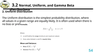
2. Uniform Distribution
The Uniform distribution is the simplest probability distribution, where
all values in a given range are equally likely. It is often used when there is
no bias or preference for any particular value.
54

55. 3.2 Normal, Uniform, and Gamma Beta
distributions
Example in Pharmacy:
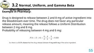
Drug is designed to release between 2 and 8 mg of active ingredient into
the bloodstream over time. The drug does not favor any particular
release amount, meaning the release follows a Uniform Distribution
between 2 mg and 8 mg.
Probability of releasing between 4 mg and 6 mg:
55

56. 3.2 Normal, Uniform, and Gamma Beta
distributions
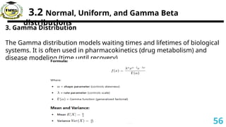
3. Gamma Distribution
The Gamma distribution models waiting times and lifetimes of biological
systems. It is often used in pharmacokinetics (drug metabolism) and
disease modeling (time until recovery).
56

57. 3.2 Normal, Uniform, and Gamma Beta
distributions
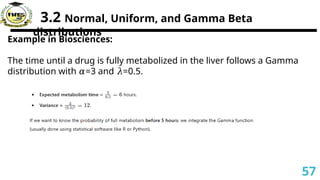
Example in Biosciences:
The time until a drug is fully metabolized in the liver follows a Gamma
distribution with =3 and =0.5.
𝛼 𝜆
57

58. 3.2 Normal, Uniform, and Gamma Beta
distributions
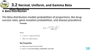
4. Beta Distribution
The Beta distribution models probabilities of proportions, like drug
success rates, gene mutation probabilities, and disease prevalence.
58

59. 3.2 Normal, Uniform, and Gamma Beta
distributions
Example in Pharmacy:
A pharmaceutical company is testing a new drug. They estimate the
probability of the drug working on a patient follows a Beta distribution
with =8 and =2.
𝛼 𝛽
59

60. 3.2 Normal, Uniform, and Gamma Beta
distributions
60

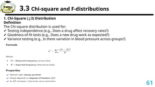
61. 3.3 Chi-square and F-distributions
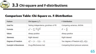
1. Chi-Square ( 2) Distribution
𝜒
Definition
The Chi-square distribution is used for:
✔ Testing independence (e.g., Does a drug affect recovery rates?)
✔ Goodness-of-fit tests (e.g., Does a new drug work as expected?)
✔ Variance testing (e.g., Is there variation in blood pressure across groups?)
61

62. 3.3 Chi-square and F-distributions
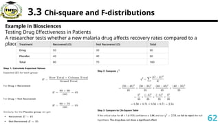
Example in Biosciences
Testing Drug Effectiveness in Patients
A researcher tests whether a new malaria drug affects recovery rates compared to a
placebo.
62

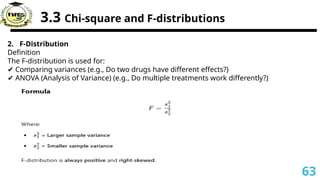
63. 3.3 Chi-square and F-distributions
2. F-Distribution
Definition
The F-distribution is used for:
✔ Comparing variances (e.g., Do two drugs have different effects?)
✔ ANOVA (Analysis of Variance) (e.g., Do multiple treatments work differently?)
63

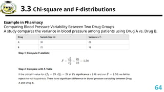
64. 3.3 Chi-square and F-distributions
Example in Pharmacy
Comparing Blood Pressure Variability Between Two Drug Groups
A study compares the variance in blood pressure among patients using Drug A vs. Drug B.
64

65. 3.3 Chi-square and F-distributions
65

66. 3.3 Chi-square and F-distributions
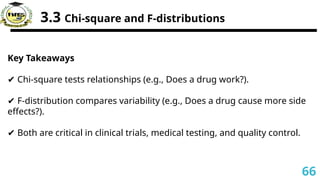
Key Takeaways
✔ Chi-square tests relationships (e.g., Does a drug work?).
✔ F-distribution compares variability (e.g., Does a drug cause more side
effects?).
✔ Both are critical in clinical trials, medical testing, and quality control.
66

67. 4. Joint Distributions and Covariance
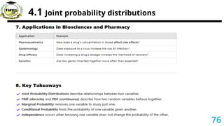
4.1 Joint probability distributions
4.2 Concept of covariance
67

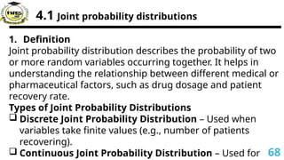
68. 4.1 Joint probability distributions
1. Definition
Joint probability distribution describes the probability of two
or more random variables occurring together. It helps in
understanding the relationship between different medical or
pharmaceutical factors, such as drug dosage and patient
recovery rate.
Types of Joint Probability Distributions
 Discrete Joint Probability Distribution – Used when
variables take finite values (e.g., number of patients
recovering).
 Continuous Joint Probability Distribution – Used for 68

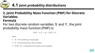
69. 4.1 Joint probability distributions
2. Joint Probability Mass Function (PMF) for Discrete
Variables
Formula
For two discrete random variables and , the joint
𝑋 𝑌
probability mass function (PMF) is:
69

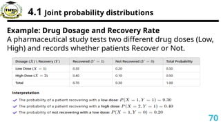
70. 4.1 Joint probability distributions
Example: Drug Dosage and Recovery Rate
A pharmaceutical study tests two different drug doses (Low,
High) and records whether patients Recover or Not.
70

71. 4.1 Joint probability distributions
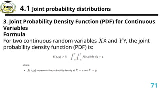
3. Joint Probability Density Function (PDF) for Continuous
Variables
Formula
For two continuous random variables X and Y, the joint
𝑋 𝑌
probability density function (PDF) is:
71

72. 4.1 Joint probability distributions
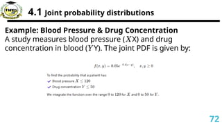
Example: Blood Pressure & Drug Concentration
A study measures blood pressure ( X) and drug
𝑋
concentration in blood ( Y). The joint PDF is given by:
𝑌
72

73. 4.1 Joint probability distributions
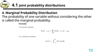
4. Marginal Probability Distribution
The probability of one variable without considering the other
is called the marginal probability.
73

74. 4.1 Joint probability distributions
Example
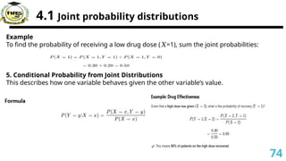
To find the probability of receiving a low drug dose ( =1), sum the joint probabilities:
𝑋
5. Conditional Probability from Joint Distributions
This describes how one variable behaves given the other variable’s value.
74

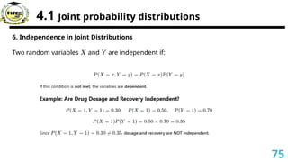
75. 4.1 Joint probability distributions
6. Independence in Joint Distributions
Two random variables and are independent if:
𝑋 𝑌
75

76. 4.1 Joint probability distributions
76

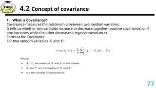
77. 4.2 Concept of covariance
1. What is Covariance?
Covariance measures the relationship between two random variables.
It tells us whether two variables increase or decrease together (positive covariance) or if
one increases while the other decreases (negative covariance).
Formula for Covariance
For two random variables and :
𝑋 𝑌
77

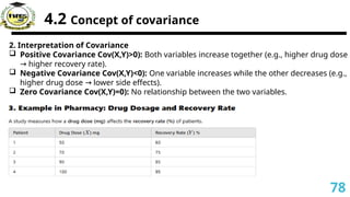
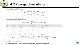
78. 4.2 Concept of covariance
2. Interpretation of Covariance
 Positive Covariance Cov(X,Y)>0): Both variables increase together (e.g., higher drug dose
higher recovery rate).
→
 Negative Covariance Cov(X,Y)<0): One variable increases while the other decreases (e.g.,
higher drug dose lower side effects).
→
 Zero Covariance Cov(X,Y)=0): No relationship between the two variables.
78

79. 4.2 Concept of covariance
79

80. 4.2 Concept of covariance
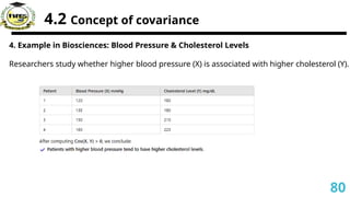
4. Example in Biosciences: Blood Pressure & Cholesterol Levels
Researchers study whether higher blood pressure (X) is associated with higher cholesterol (Y).
80

81. 4.2 Concept of covariance
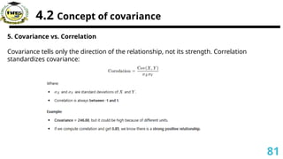
5. Covariance vs. Correlation
Covariance tells only the direction of the relationship, not its strength. Correlation
standardizes covariance:
81

82. 4.2 Concept of covariance
82

83. 5. Sampling and Estimation
5.1 Sampling methods and distributions
5.2 Sample size calculations
5.3 Confidence intervals
83

84. 5.1 Sampling methods and distributions
84

85. 5.1 Sampling methods and distributions
85

86. 5.1 Sampling methods and distributions
86

87. 5.1 Sampling methods and distributions
87

88. 5.1 Sampling methods and distributions
88

89. 5.1 Sampling methods and distributions
89

90. 5.2 Sample size calculations
90

91. 5.2 Sample size calculations
91

92. 5.2 Sample size calculations
92

93. 5.2 Sample size calculations
93

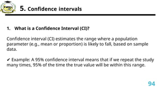
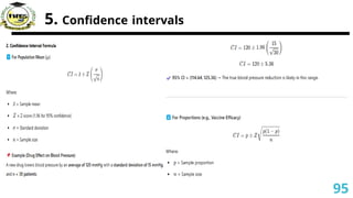
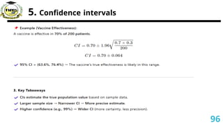
94. 5. Confidence intervals
1. What is a Confidence Interval (CI)?
Confidence interval (CI) estimates the range where a population
parameter (e.g., mean or proportion) is likely to fall, based on sample
data.
✔ Example: A 95% confidence interval means that if we repeat the study
many times, 95% of the time the true value will be within this range.
94

95. 5. Confidence intervals
95

96. 5. Confidence intervals
96

97. 6. Hypothesis Testing
6.1 Errors in hypothesis testing
6.2 Decision rules for hypothesis testing
97

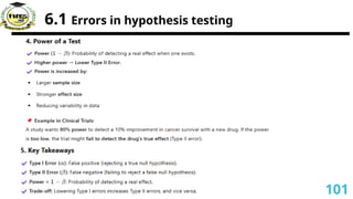
98. 6.1 Errors in hypothesis testing
1. What is Hypothesis Testing?
Hypothesis testing is a statistical method to make decisions about a
population based on sample data. It involves:
 Null Hypothesis ( 0​
)
𝐻 – Assumes no effect or no difference (e.g., "A
drug has no effect").
 Alternative Hypothesis ( )
𝐻𝐴 – Suggests a real effect or difference
(e.g., "A drug lowers blood pressure").
 Decision Making – Based on a p-value and a chosen significance
level ( )
𝛼
(e.g., 0.05).
98

99. 6.1 Errors in hypothesis testing
99

100. 6.1 Errors in hypothesis testing
100

101. 6.1 Errors in hypothesis testing
101

102. 6.2 Decision rules for hypothesis testing
102

103. 6.2 Decision rules for hypothesis testing
103

104. 6.2 Decision rules for hypothesis testing
104

105. 105
THANK YOU