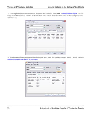
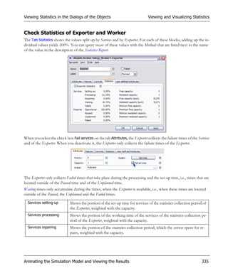
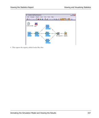
Downloaded 461 times


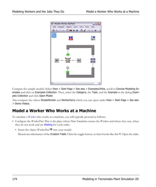
![Finding Objects and Text in Your Simulation Model Working with the Program, Basics
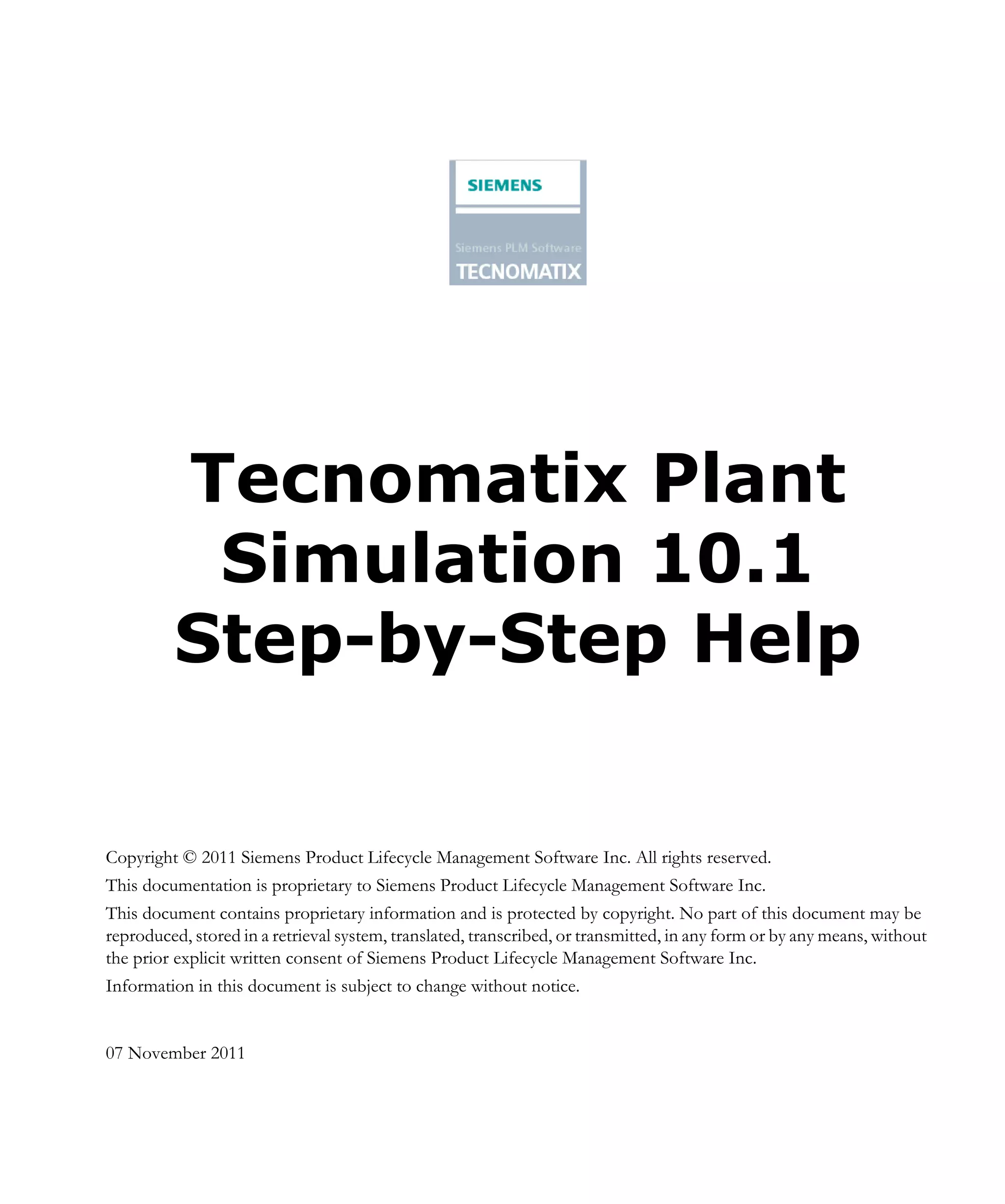
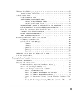
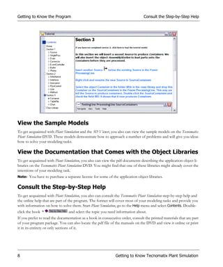
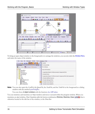
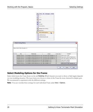
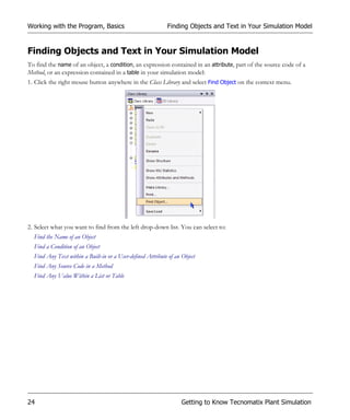
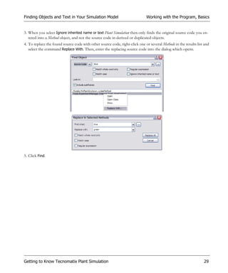
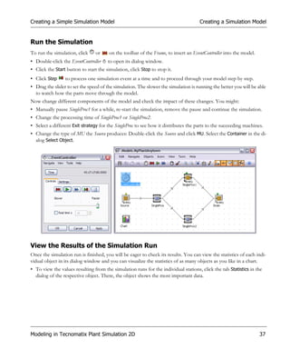
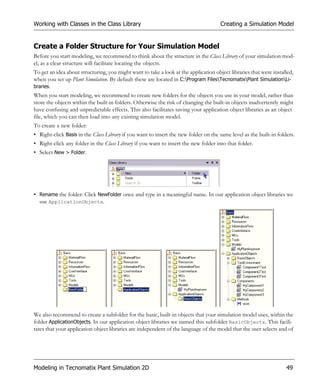
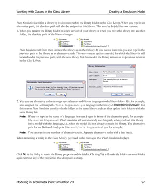
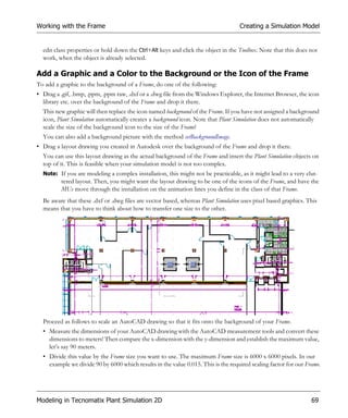
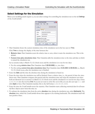
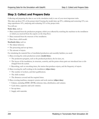
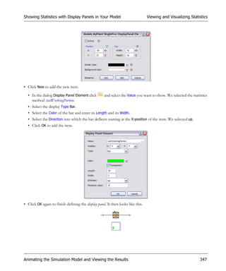
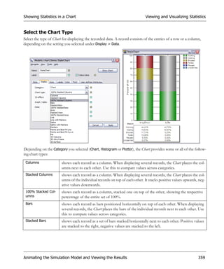
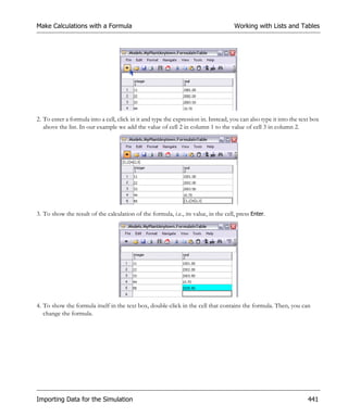
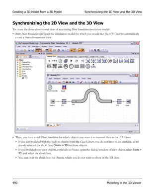
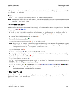
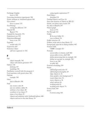
Select To enter and to find
One or more matches +
Any one character in the set []
Any one character not in the set [^]
Or |
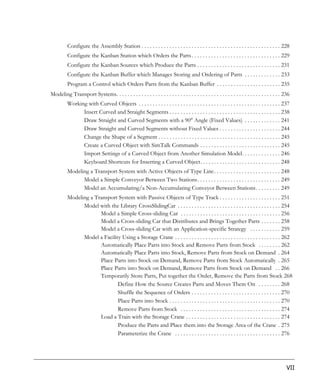
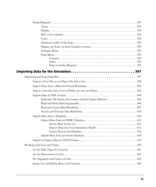
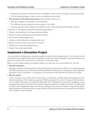
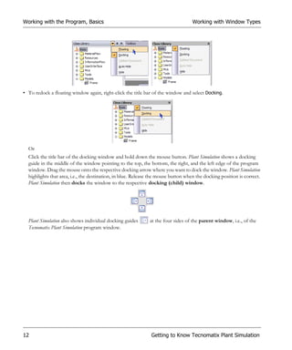
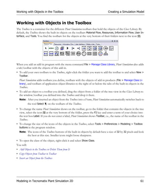
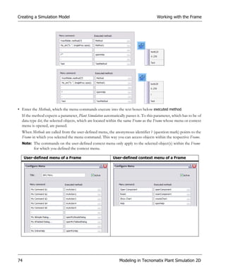
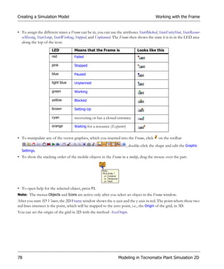
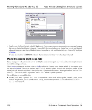
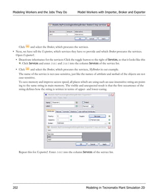
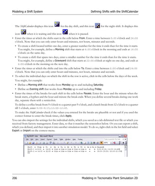
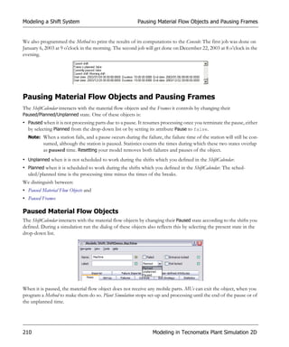
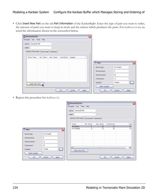
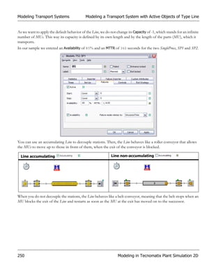
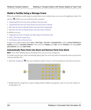
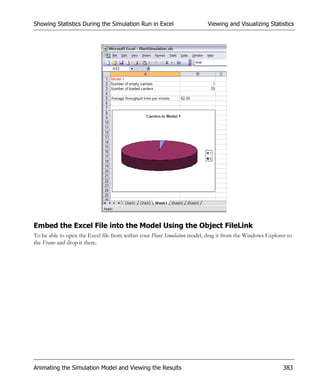
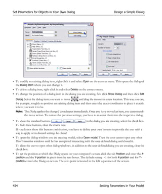
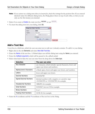
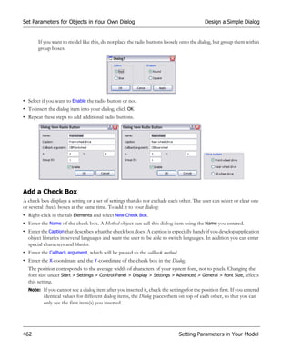
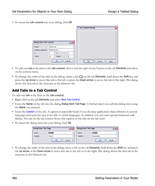
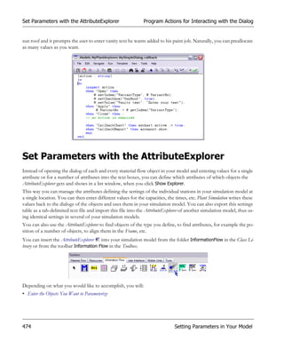
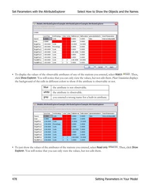
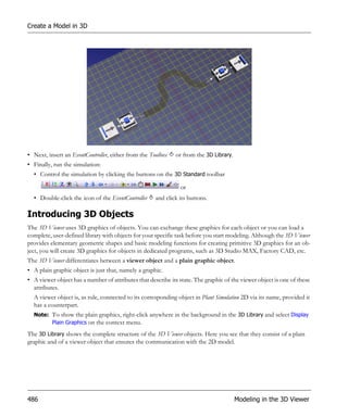
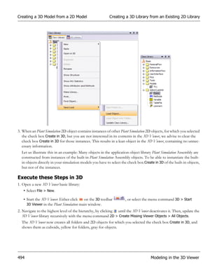
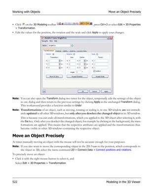
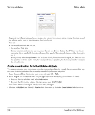
Searching with regular expressions allows you to use wild cards in the string you are searching for.
• To find all strings that contain a sequence of the character a, followed by any character, and the character b,
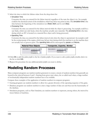
enter a.b into the text box.
• To find all objects whose name starts with an upper case S, enter ^[S].
• To find all objects whose name does not end with an e, enter [^e]$.
• To find all objects whose name contains an upper case L, followed by any character, followed by proc, enter
L.*proc into the text box.
11.Click Find.
Find a Condition of an Object
To find a condition of an object you inserted into your simulation model:
1. Select Condition from the left drop-down list.
2. Enter any SimTalk expression whose attributes or methods are identical to the expression you enter in the drop-
down combo box. You might, for example, enter the name of an attribute or a method and the expression you are
looking for, such as Proctime = 100, or OpenCtrl = void, etc.
3. Repeat steps 4 to 7 described under Find the Name of an Object.
4. Click Find.
Getting to Know Tecnomatix Plant Simulation 27](https://image.slidesharecdn.com/plantsimulationstep-by-stepenu-130104132843-phpapp02/85/Plant-Simulation-Passo-a-Passo-47-320.jpg)
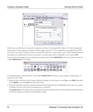
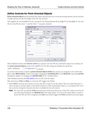
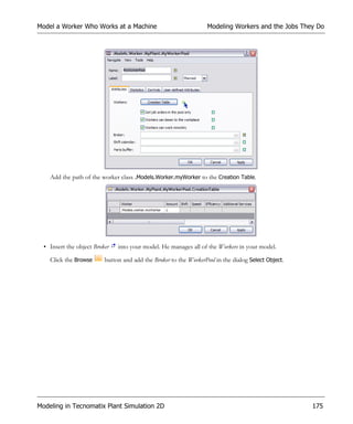
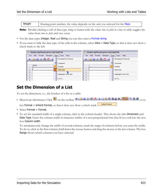
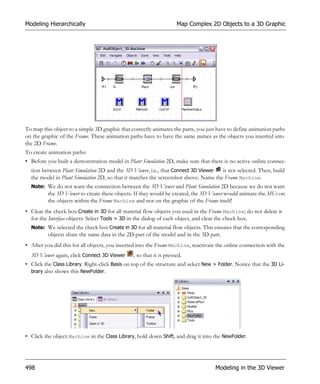
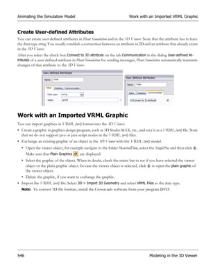
![Working with the Frame Creating a Simulation Model
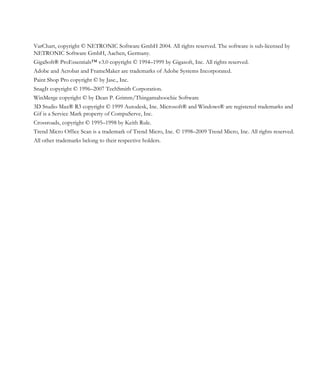
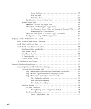
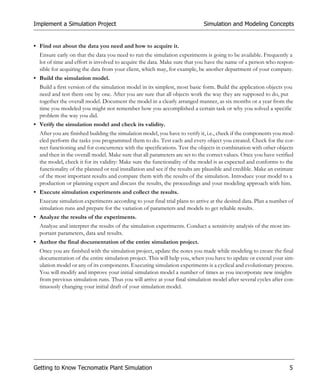
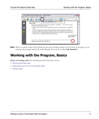
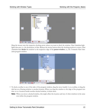
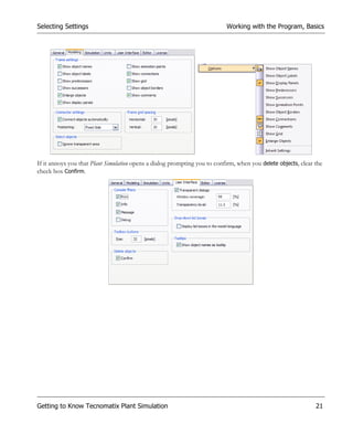
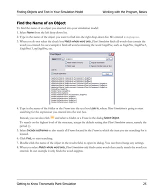
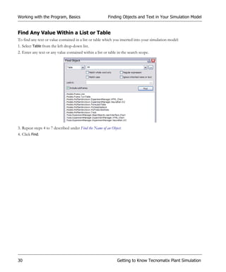
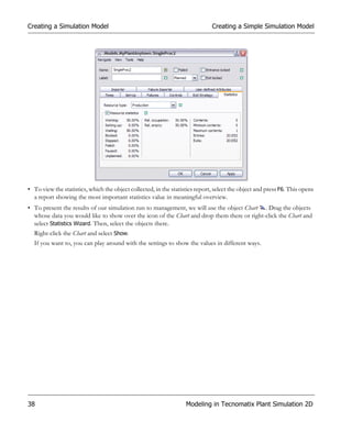
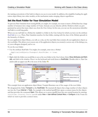
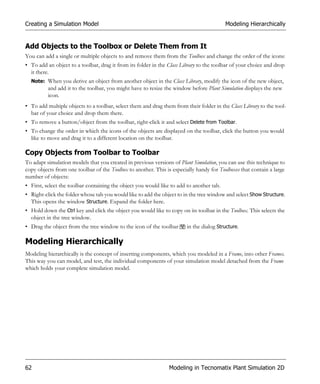
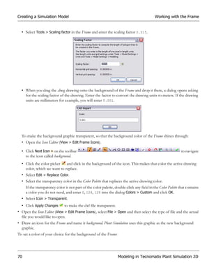
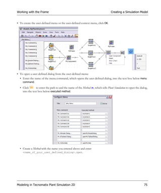
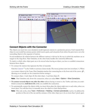
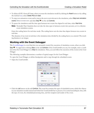
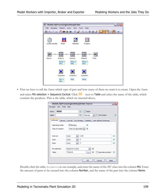
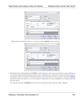
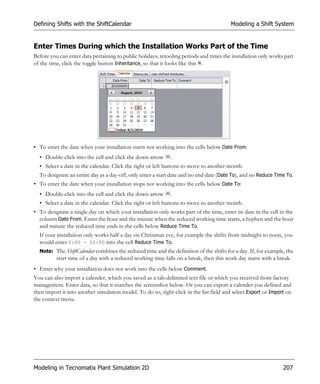
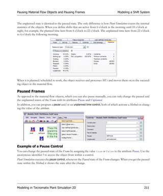
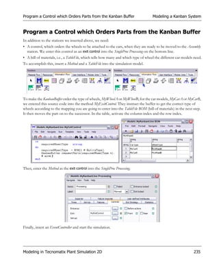
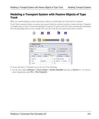
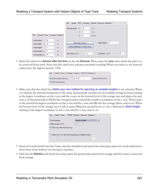
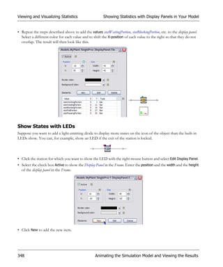
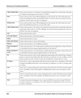
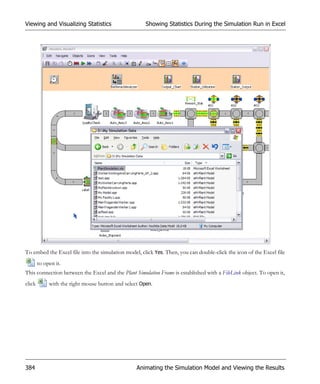
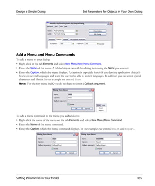
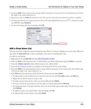
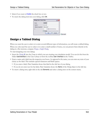
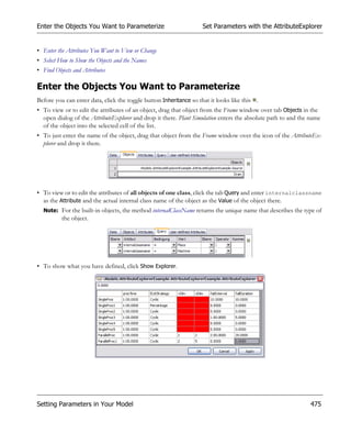
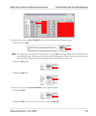
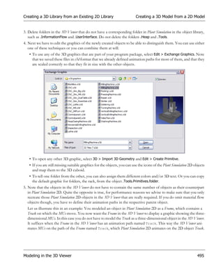
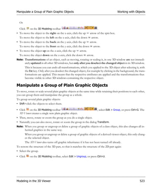
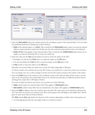
Note: To create a user-defined menu in a Frame, which you inserted into another Frame, deactivate the menu
command Inherit, so that it does not show a check mark to the left.
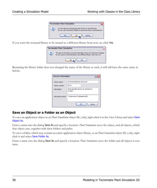
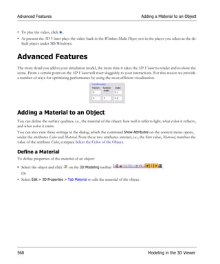
• Enter the Title of the User-defined Menu with which Plant Simulation shows the menu next to the built-in menu bar
of the Frame.
• To show the User-defined Menu below the built-in menu bar of the Frame, for which you defined it, select Active.
• Enter the name of the menu command that Plant Simulation shows on the User-defined Menu in the Frame. Enter an
& (ampersand) in front of a letter to make this letter the access key. You can select this menu command by hold-
ing down the Alt key and by pressing that letter. The built-in Plant Simulation access keys take precedence over
any access keys you define!
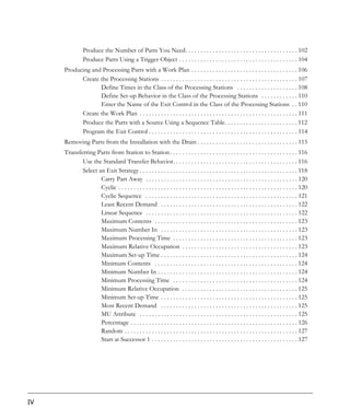
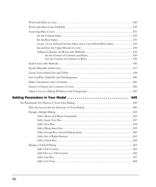
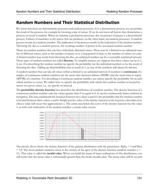
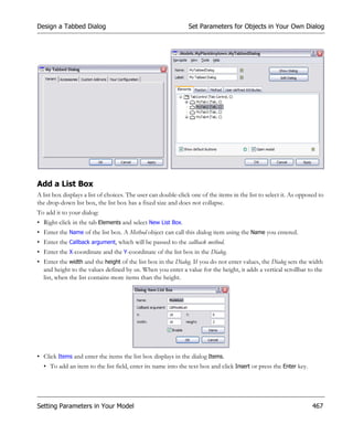
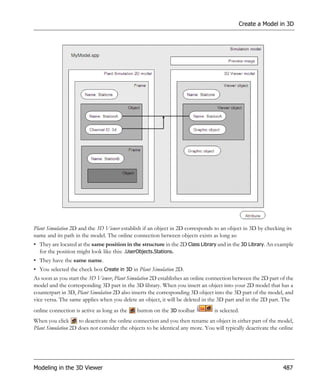
You can also enter a formula as a menu command. A formula is designated by a leading question mark. When
you enter ?Method1 for example, the method Method1 will be called. The return value of this method has to be
of data type string. This way you can toggle between different texts, for example between Activate and Deactivate
and you can translate the menu commands into different languages. If the methods return an empty string (""),
Plant Simulation hides the respective menu command.
Note: You can use any formulas, even for example a method call with parameters, such as ?Method1(42) or a
table access, such as ?TableFile[1,3].
Modeling in Tecnomatix Plant Simulation 2D 73](https://image.slidesharecdn.com/plantsimulationstep-by-stepenu-130104132843-phpapp02/85/Plant-Simulation-Passo-a-Passo-93-320.jpg)
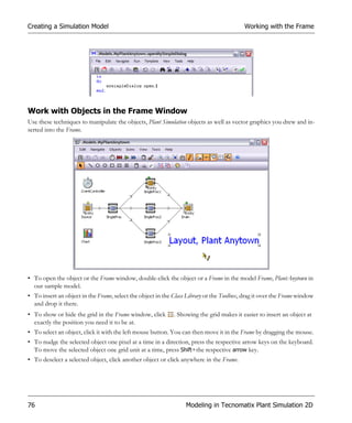
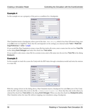
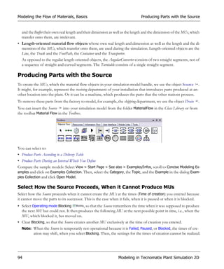
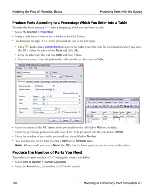
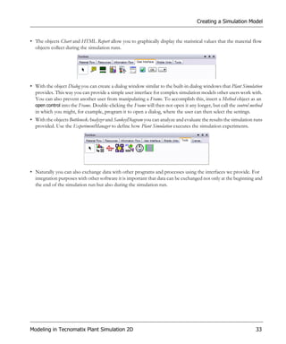
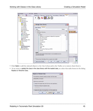
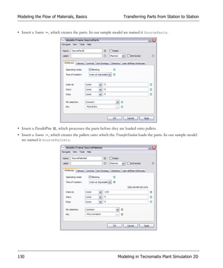
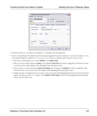
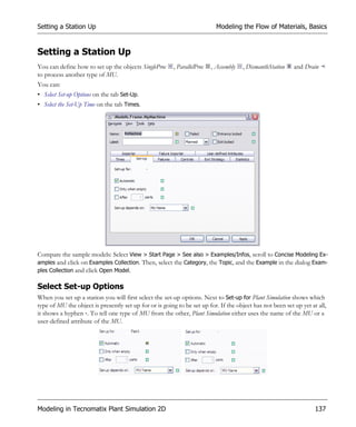
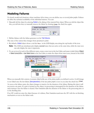
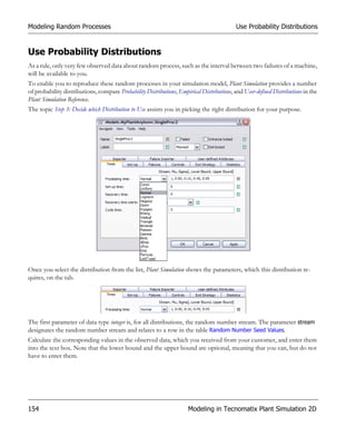
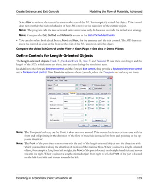
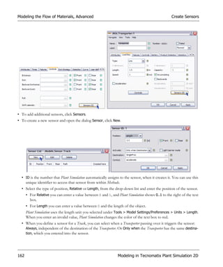
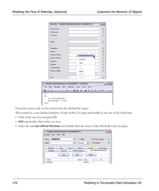
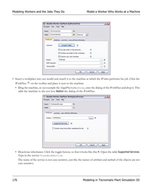
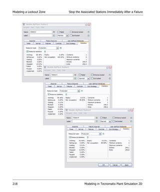
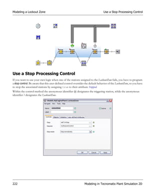
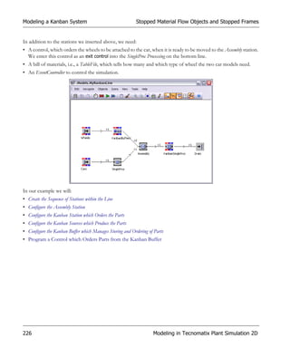
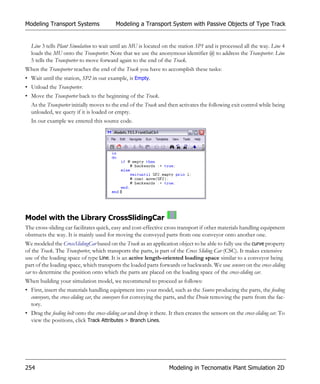
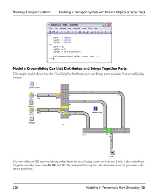
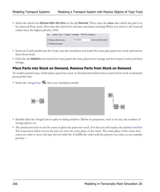
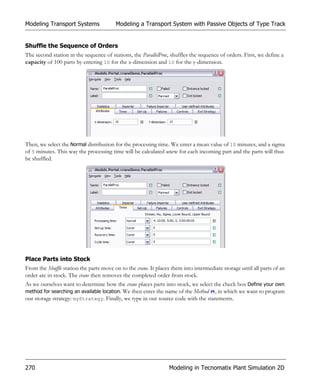
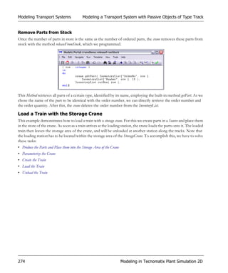
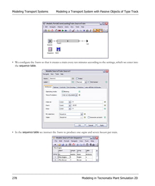
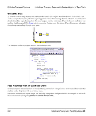
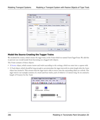
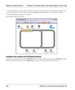
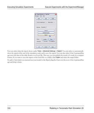
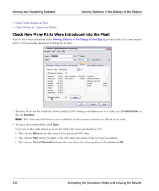
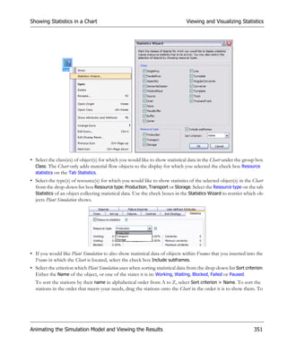
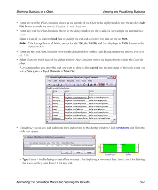
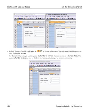
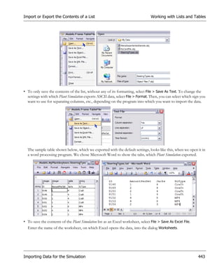
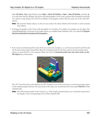
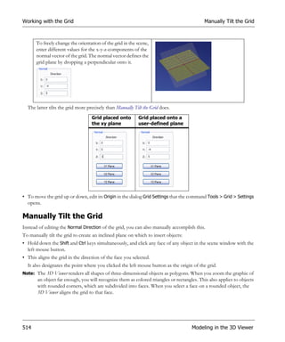
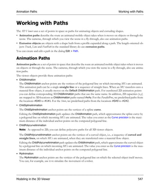
![Producing Parts with the Source Modeling the Flow of Materials, Basics
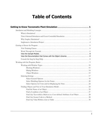
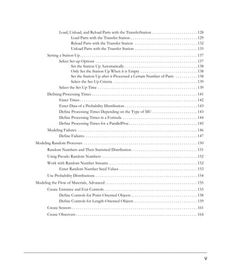
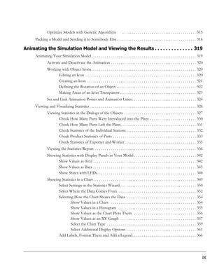
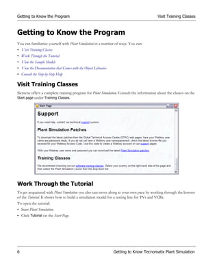
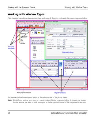
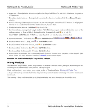
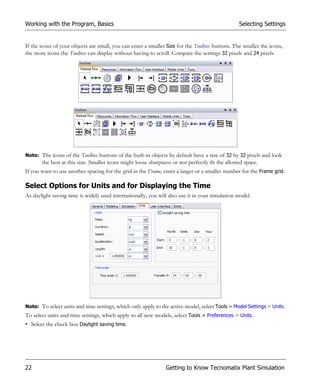
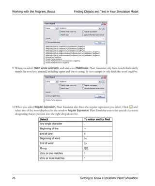
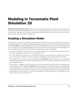
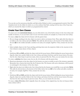
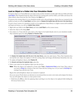
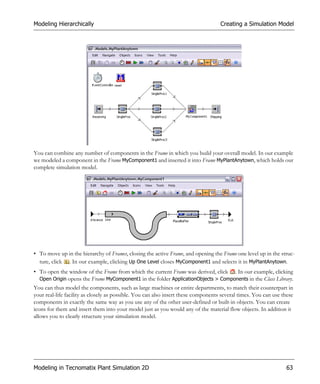
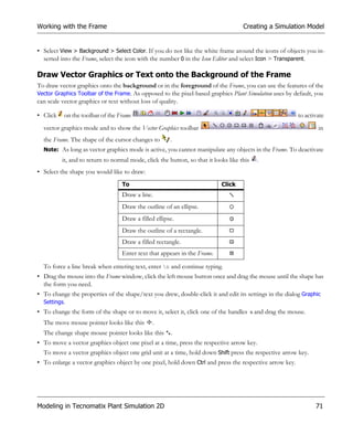
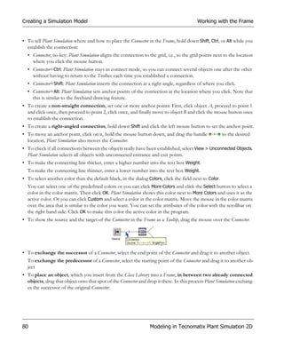
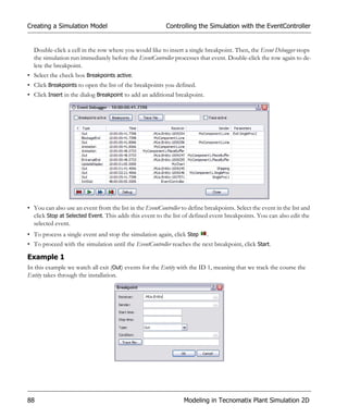
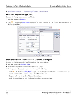
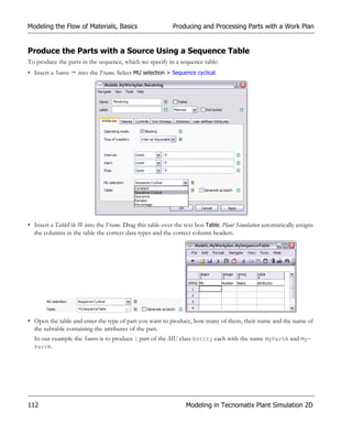
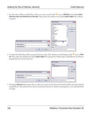
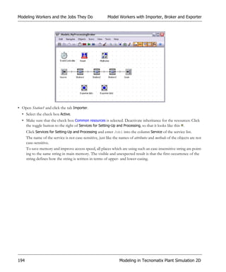
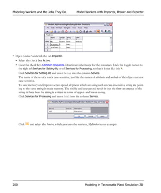
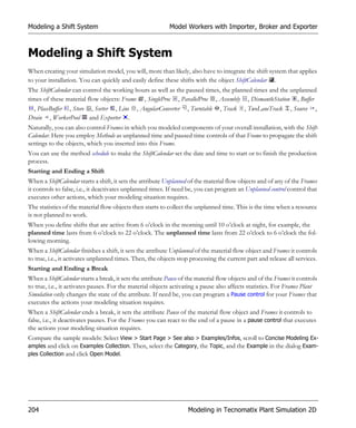
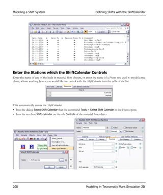
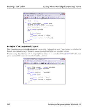
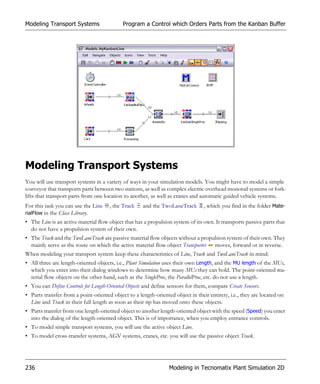
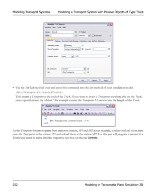
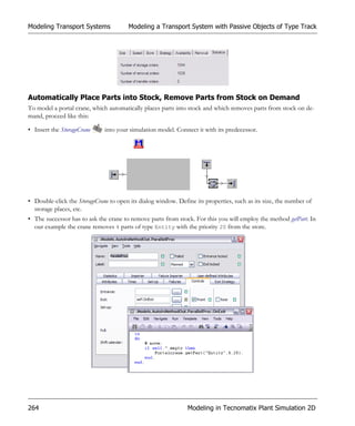
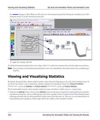
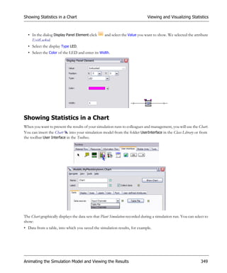
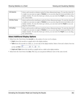
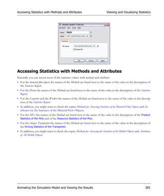
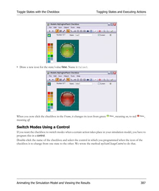
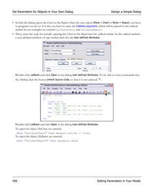
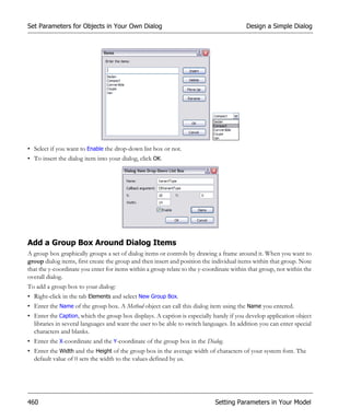
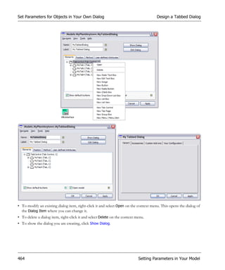
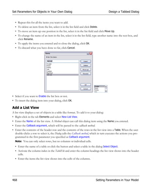
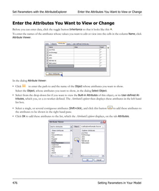
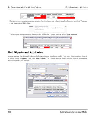
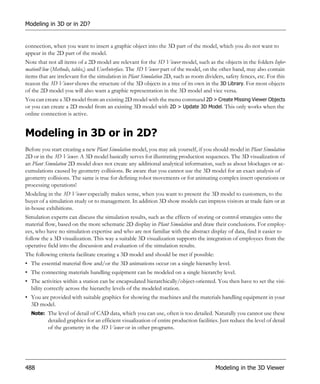
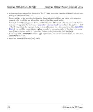
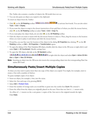
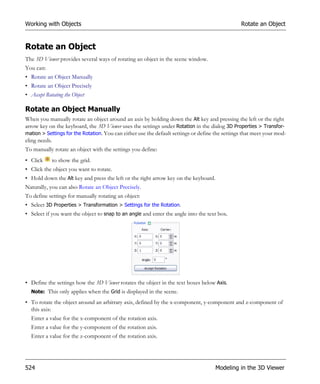
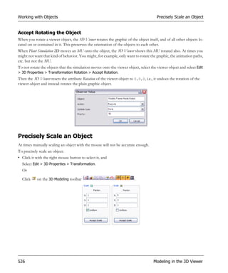
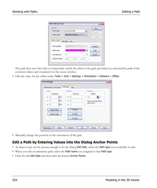
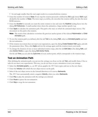
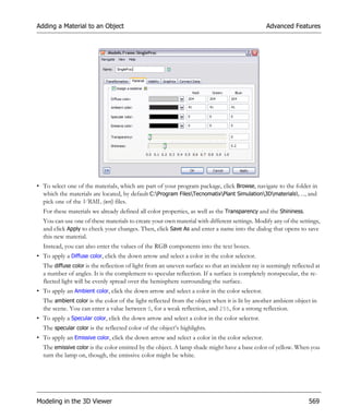
• Click the tab Values and select the Trigger type > Input.
• Click the button Values and enter into the TimeSequence object that opens:
The Point in Time at which the Source creates MUs into the cells on the left hand side.
The current sequence of Values into the cells on the right hand side. An order is a string with this format:
<amount>,<mu_Type>,<distributionType>,<stream>[,<distribution parameters>].
Note: The string defining this sequence of values may not contain any blank spaces.
You have to enter the amount of MUs to be produced, the type to be produced, and at least a constant value.
When you enter just Const, the Source produces the MUs at the point in time, which you entered into the cell to
the left. When you would like it to produce the MUs with an offset to the time you entered there, enter the num-
ber of seconds after which it produces them after Const.
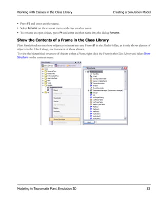
When you enter a distribution, its values set the time offset to the time you entered into the corresponding left
cell. Note that the offset you enter has to be a positive number!
Modeling in Tecnomatix Plant Simulation 2D 105](https://image.slidesharecdn.com/plantsimulationstep-by-stepenu-130104132843-phpapp02/85/Plant-Simulation-Passo-a-Passo-125-320.jpg)
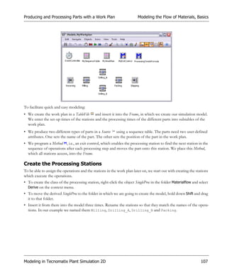
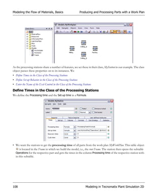
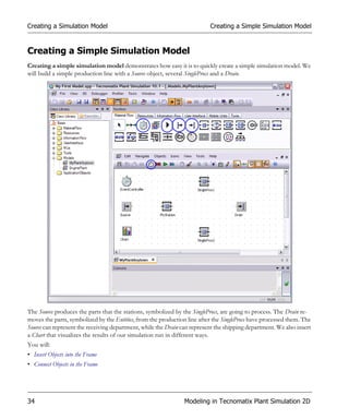
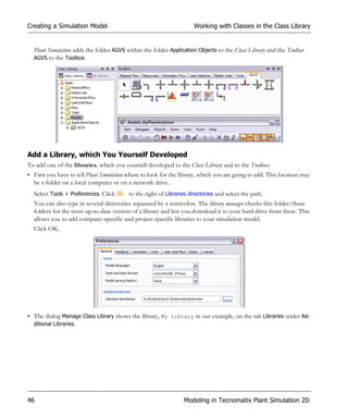
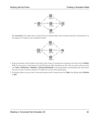
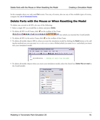
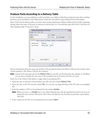
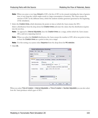
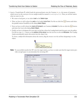
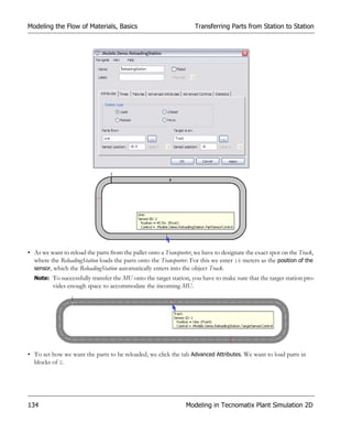
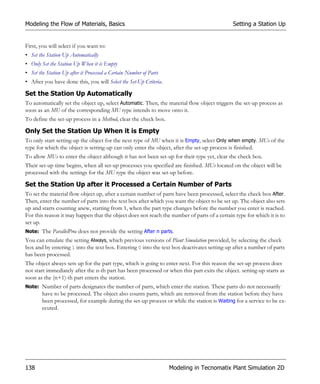
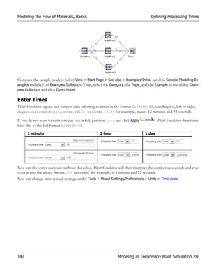
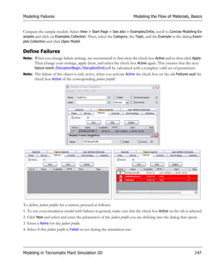
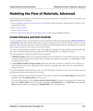
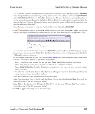
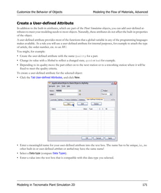
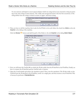
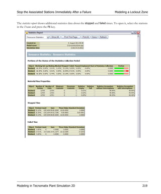
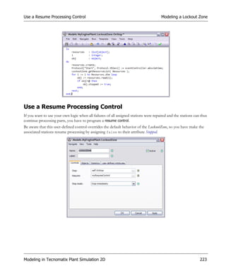
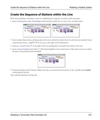
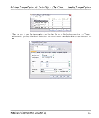
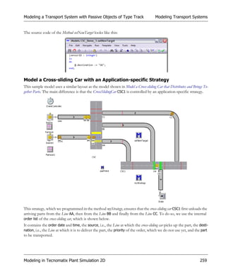
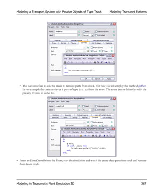
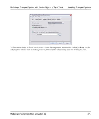
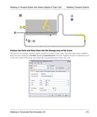
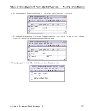
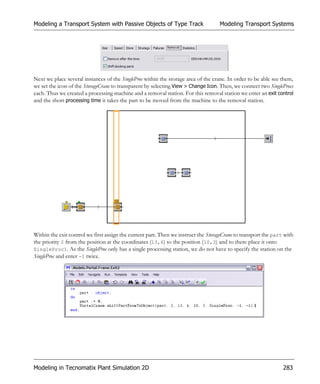
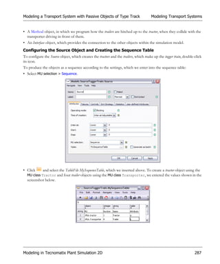
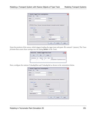
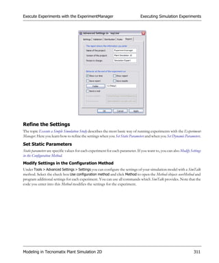
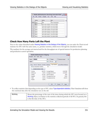
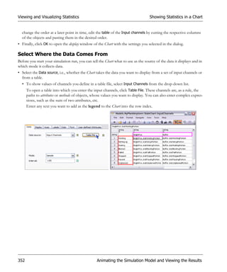
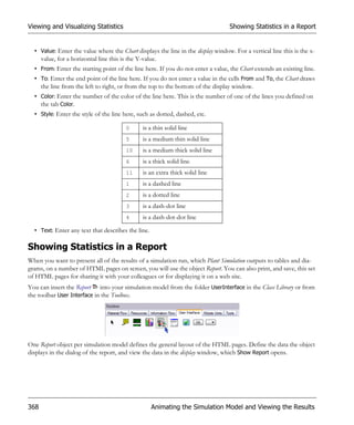
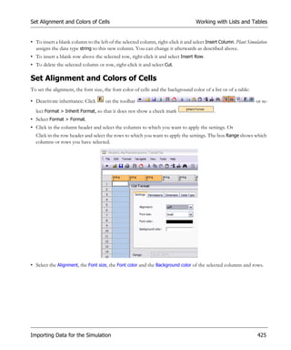
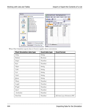
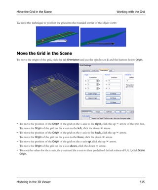
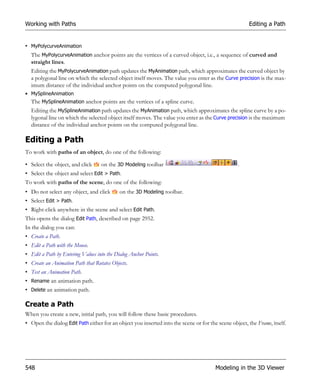
![Producing and Processing Parts with a Work Plan Modeling the Flow of Materials, Basics
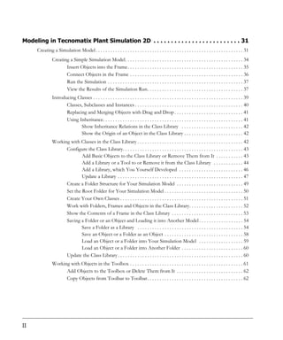
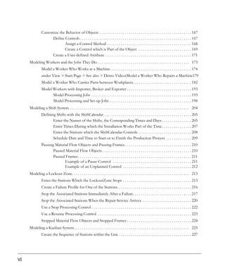
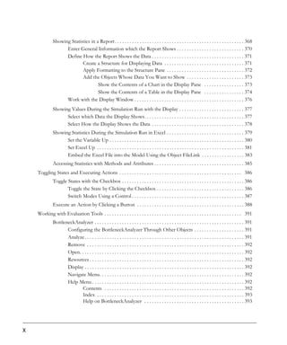
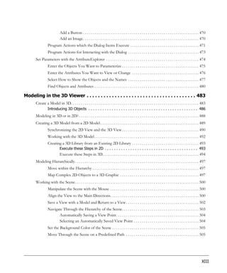
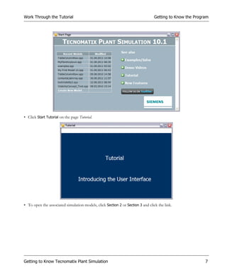
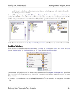
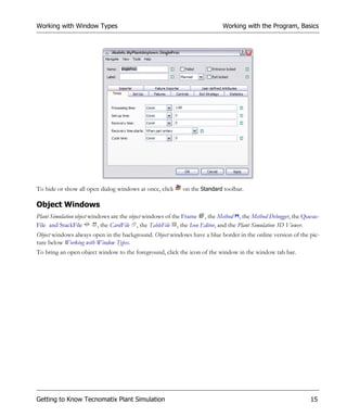
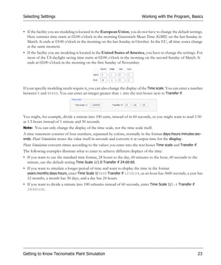
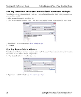
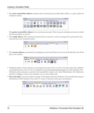
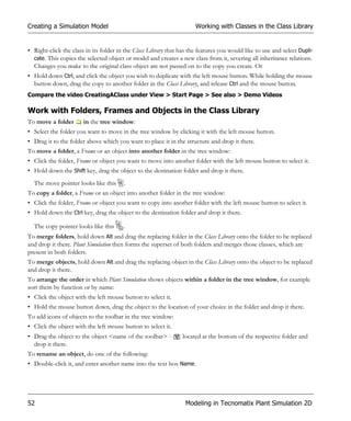
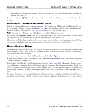
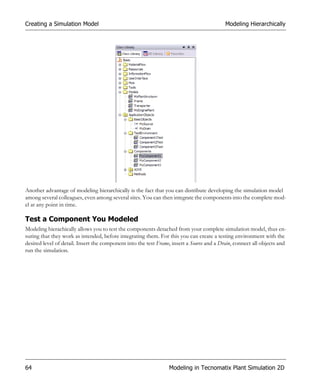
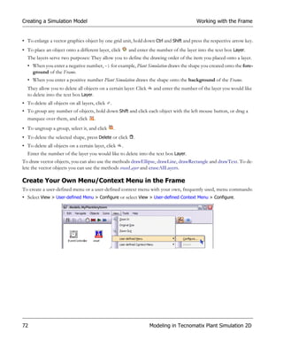
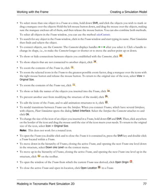
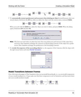
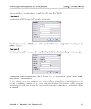
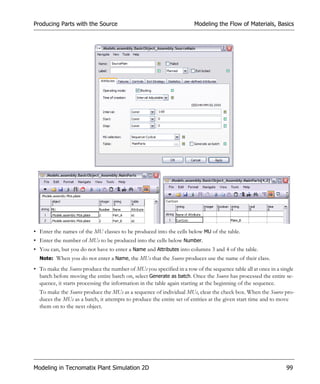
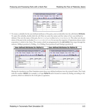
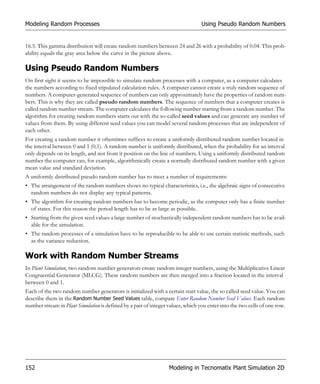
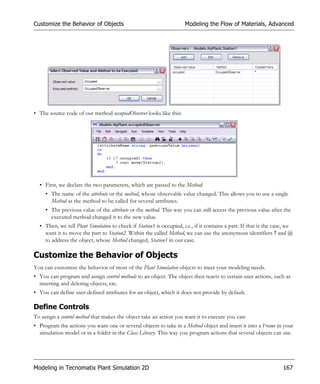
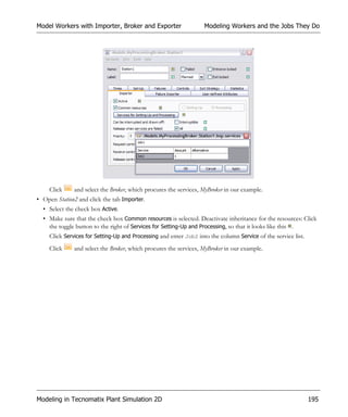
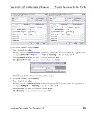
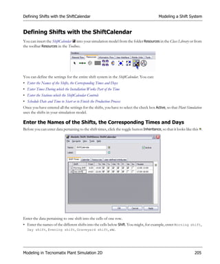
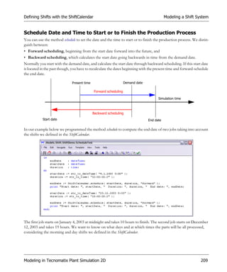
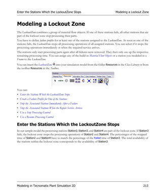
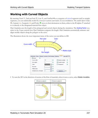
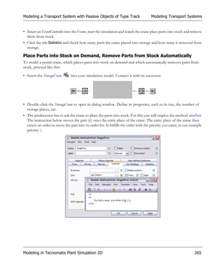
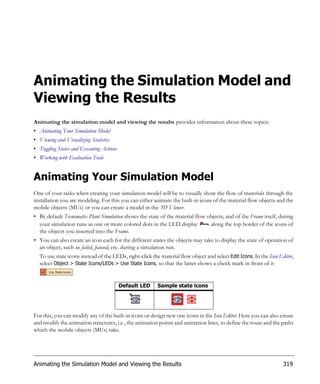
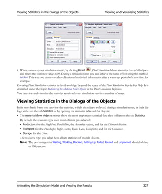
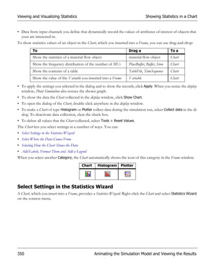
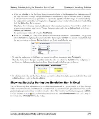
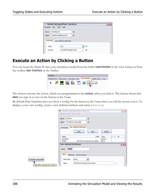
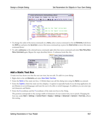
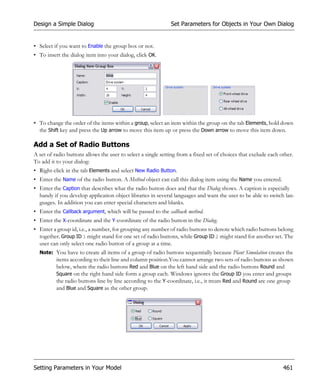
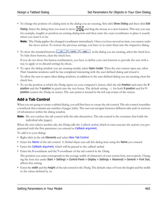
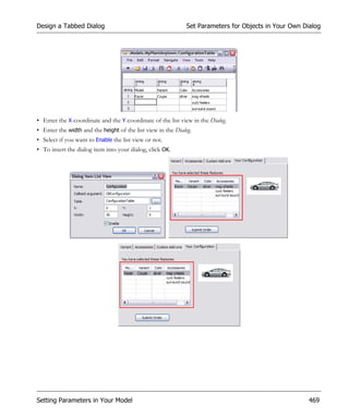
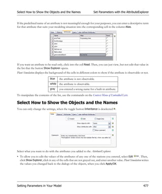
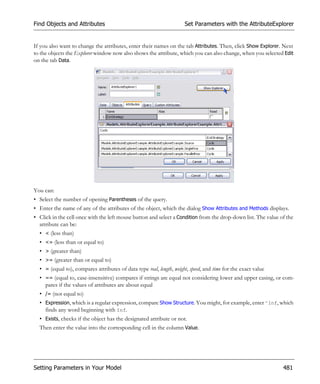
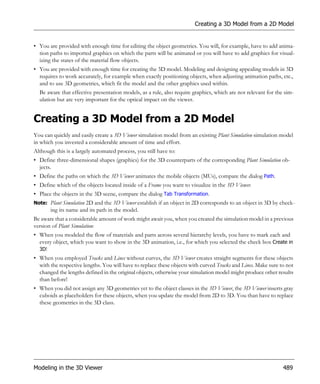
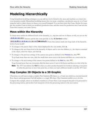
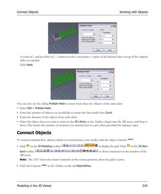
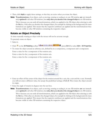
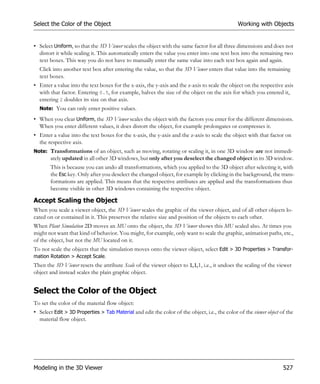
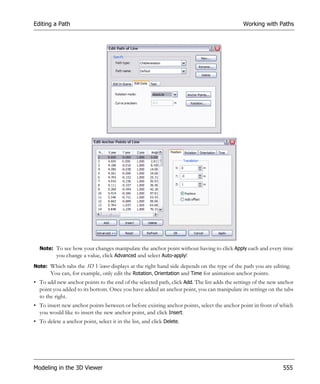
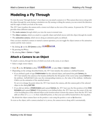
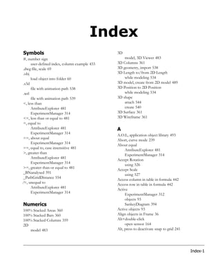
For the processing time we use a formula, which we programmed in the Method processingTimeInFormula.
• We want the stations to get the set-up time of all parts from the work plan MyWorkPlan. This table object is
located in the Frame in which we build the model, i.e., the root frame. The station then opens the subtable Opera-
tions for the respective part and gets the times in the column Set-up time of the respective station within this
subtable. Self identifies the station contained in the row in the subtable.
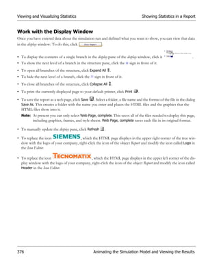
The above statements translate into this formula, which we directly enter into the text box:
root.MyWorkPlan["Operations",@.EntityType]["Setup time",Self]
Modeling in Tecnomatix Plant Simulation 2D 109](https://image.slidesharecdn.com/plantsimulationstep-by-stepenu-130104132843-phpapp02/85/Plant-Simulation-Passo-a-Passo-129-320.jpg)
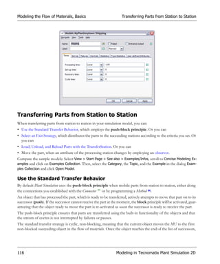
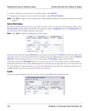
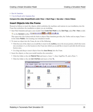
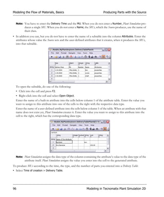
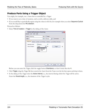
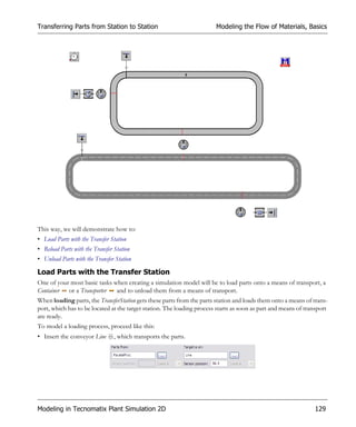
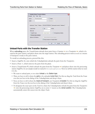
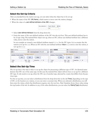
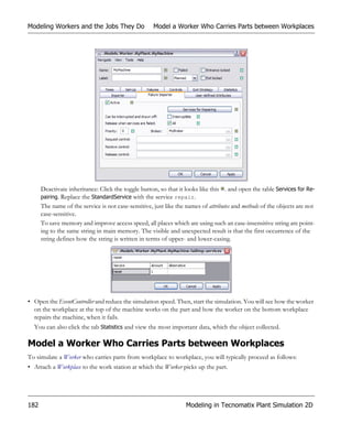
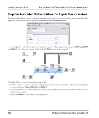
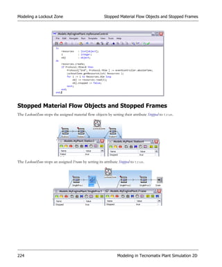
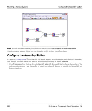
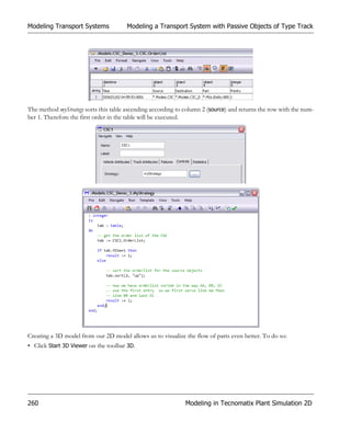
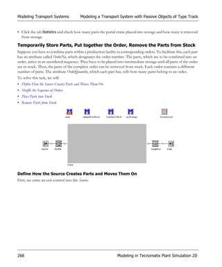
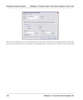
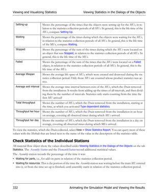
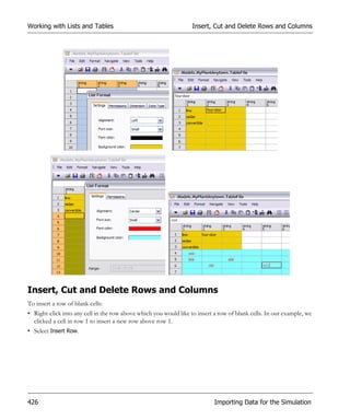
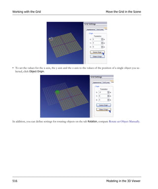
![Modeling the Flow of Materials, Basics Transferring Parts from Station to Station
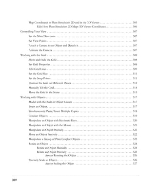
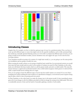
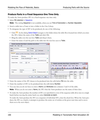
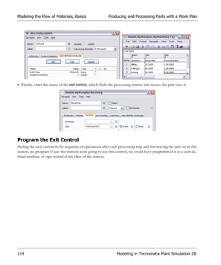
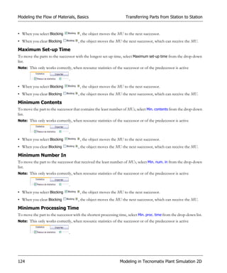
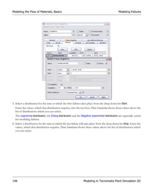
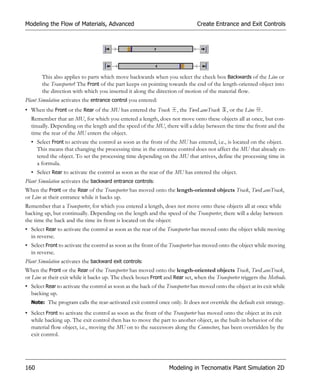
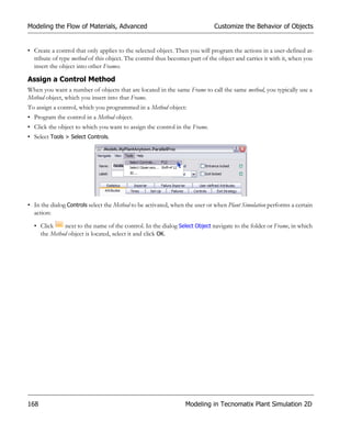
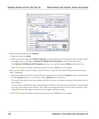
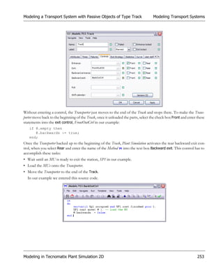
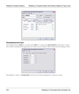
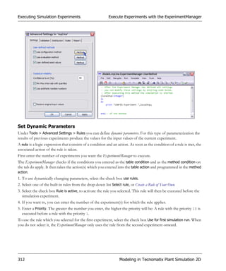
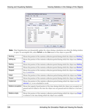
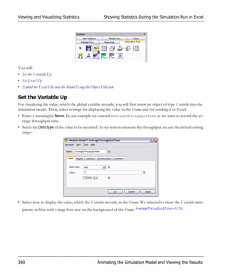
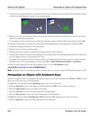
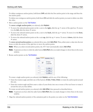
Percentage
To move the part to the successors according to a percentage distribution, select Percentage from the drop-down
list.
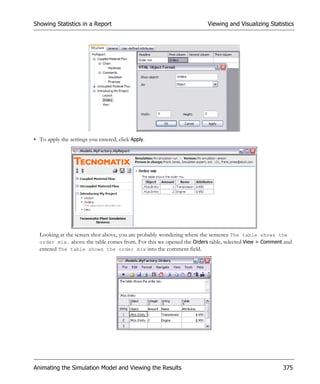
Note: Click Apply, to apply your settings, and to display the button Open List.
Click Open List and enter the percentages in the list that opens. The n-th row in the table defines the n-th successor’s
portion: When you enter 20 in row 1, for example, the object moves 20% of the MUs it received to the successor
with the number 1, etc.
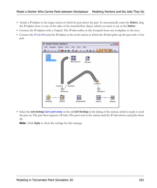
The object always moves the MU to the successor with the greatest difference between the rated value and the cur-
rent value.
• When you select Blocking , it moves the MU to the successor with the highest deviation from the nom-
inal percentage.
• When you clear Blocking , it moves the MU to the successor, which can receive the MU with the highest
deviation from the nominal percentage.
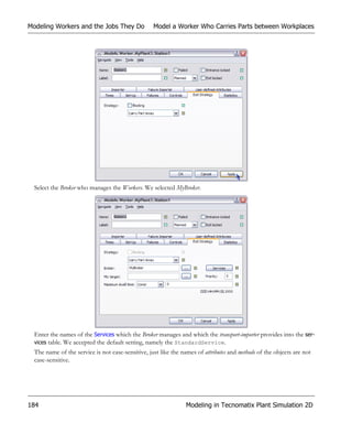
Note: The actual percentages reached may differ from the nominal ones due to a low number of total transfers
and to the Blocking-state of successors.
Any previous transfers of MUs affect the Percentage strategy, as they alter the deviation from the nominal
transfer frequencies.
Plant Simulation sums up the values you entered into the list of nominal percentages to obtain the value that matches
100%. The distribution pattern only depends on the relative size of the values, not on their magnitude. This way
you can, for example, either enter [1;2] or [0.3333…; 0.6666…], the result will be the same.
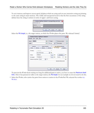
126 Modeling in Tecnomatix Plant Simulation 2D](https://image.slidesharecdn.com/plantsimulationstep-by-stepenu-130104132843-phpapp02/85/Plant-Simulation-Passo-a-Passo-146-320.jpg)
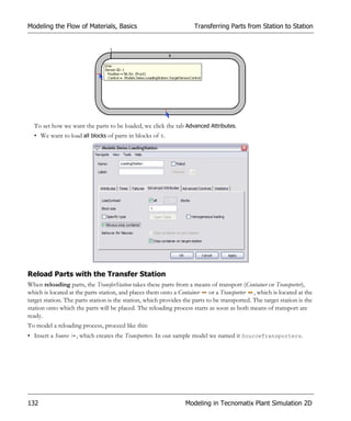
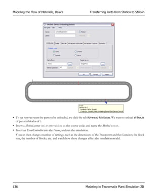
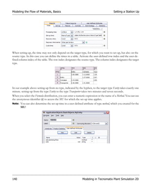
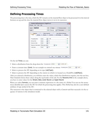
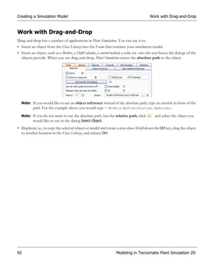
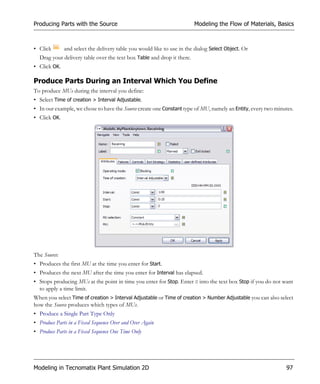
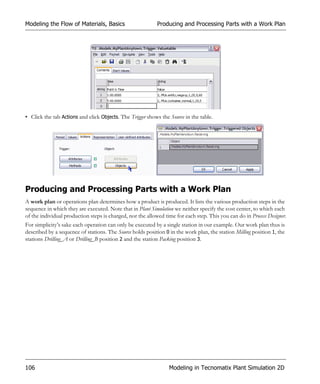
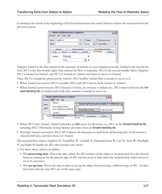
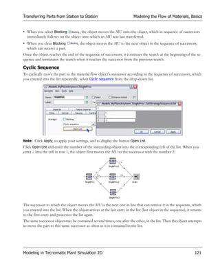
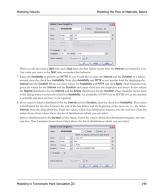
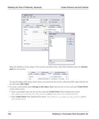
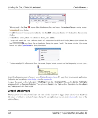
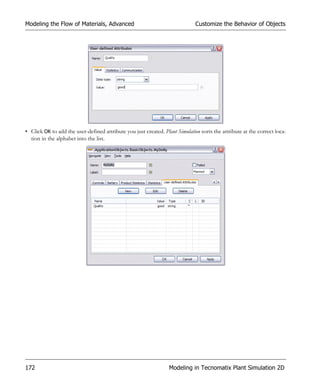
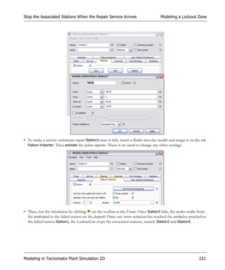
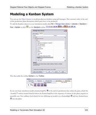
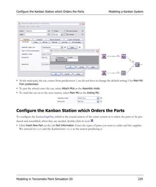
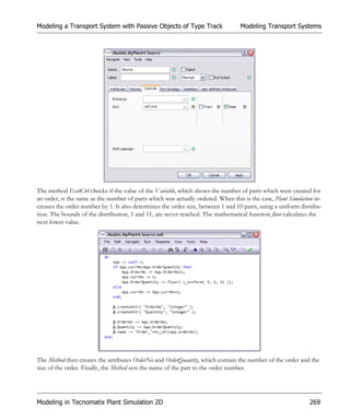
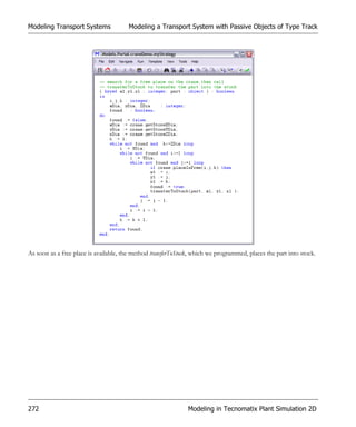
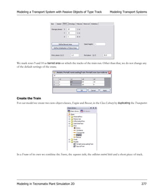
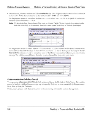
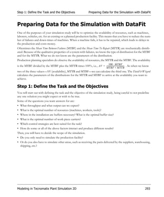
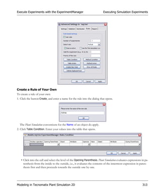
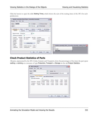
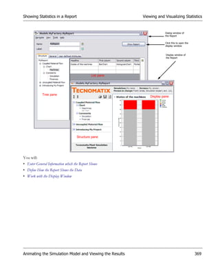
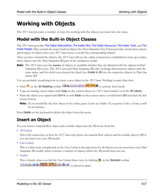
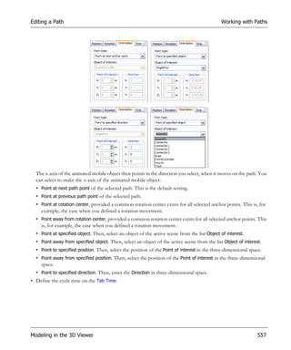
![Defining Processing Times Modeling the Flow of Materials, Basics
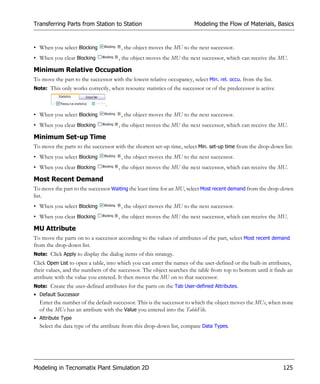
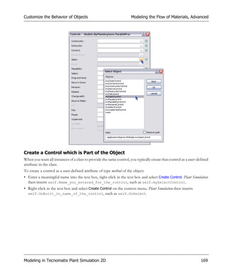
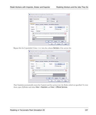
In our example, the formula, which we entered into the method cyclesMethod, sets how long the station processes the
MUs in accordance to their color.
To set the processing time of a station in a formula with an arithmetic operator:
• Select Formula as the Processing time.
• Enter the expression into the text box. In our example we entered x+2. x is the name of an object of type Variable,
of data type time. This variable adds two minutes to the processing time.
To set the processing time of a station by accessing the MU:
• Enter @.timeRed into the text box.
• Create a user-defined attribute for the MU and name it timeRed.
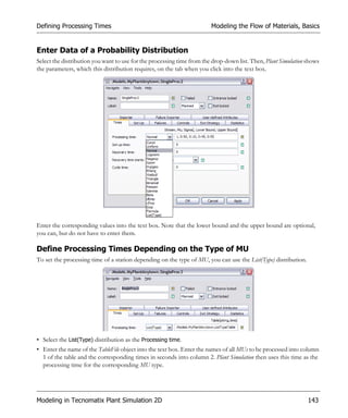
Define Processing Times for a ParallelProc
To set the processing time of a ParallelProc with several processing stations, which have different but constant
processing times, you can use the List(Place) distribution.
• Select the List(Place) distribution as the Processing time.
• Enter the name of the TableFile object into the text box. In this table, the entry [1,2] corresponds to the process-
ing station located at position [1,2], for example.
When an MU arrives at a processing station of a ParallelProc during a simulation run, Plant Simulation takes the
appropriate time for that station from the table.
Modeling in Tecnomatix Plant Simulation 2D 145](https://image.slidesharecdn.com/plantsimulationstep-by-stepenu-130104132843-phpapp02/85/Plant-Simulation-Passo-a-Passo-165-320.jpg)
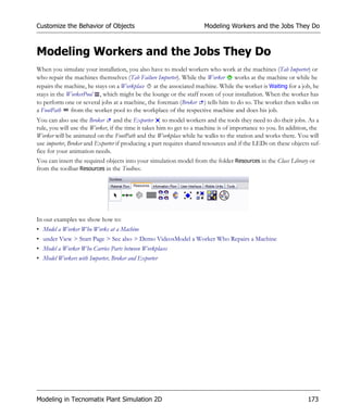

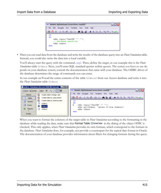
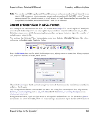
![Import Data in XML Format Importing and Exporting Data
Read and Access Data Randomly
You can read the data in its entirety, and then randomly process it as a whole. Here Plant Simulation imports the
entire document first and then processes and analyzes all data in the Method, which you program. Randomly access-
ing data requires that all data you want to use is in RAM. The larger the amount of data, the more RAM the XM-
LInterface uses!
You might, for example:
• Select data from the XML document.
-- randomly accesses data via XPath instructions
is
tbl:table;
do
XMLInterface.filename := "D:MSXML 4.0books.xml";
-- load the XML document for random access into RAM
XMLInterface.openDocument;
-- select nodes via XPath instruction
-- selection starts at the Context node which you entered in the XMLInterface
-- the second parameter is the selection depth for each node
-- 0 means that no children will be selected
-- the result is passed to a table
tbl := XMLInterface.getNodes("book[title='Midnight Rain']", 1);
XMLInterface.close;
end;
• Delete existing data from the XML document.
-- deletes all nodes specified by XPath instructions
is
do
XMLInterface.filename := "D:MSXML 4.0books.xml";
-- load the XML document for random access into the RAM
XMLInterface.openDocument;
-- delete all book nodes of genre 'Fantasy'
XMLInterface.deleteNodes("book[genre = 'Fantasy']");
XMLInterface.filename := "D:MSXML 4.0tmp.xml";
-- write the document to a file
XMLInterface.write;
-- remove the document from RAM
XMLInterface.close;
end;
• Insert new data into the XML document.
-- inserts new data into the XML document
is
tbl:table;
do
Importing Data for the Simulation 407](https://image.slidesharecdn.com/plantsimulationstep-by-stepenu-130104132843-phpapp02/85/Plant-Simulation-Passo-a-Passo-427-320.jpg)
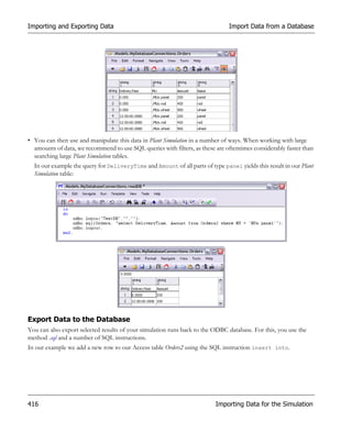
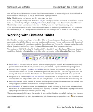
![Importing and Exporting Data Import Data in XML Format
XMLInterface.filename := "D:MSXML 4.0books.xml";
-- load the XML document
XMLInterface.openDocument;
-- get an empty table for writing the data to
-- depth=1 means that we want to write nodes with children
tbl := XMLInterface.getContainer(1);
-- set the parent node for the new data
XMLInterface.setContext("/catalog");
-- designate the node to append to the 'catalog' nodes
tbl[1,1] := "book";
-- are the attributes of the 'book' node
tbl.createNestedList(4,1);
-- explicit namespace
tbl[4,1][1,1] := "xmlns:aa";
tbl[4,1][2,1] := "specAth";
-- additional attributes
tbl[4,1][1,2] := "id";
tbl[4,1][2,2] := "bk113";
-- child nodes
tbl.createNestedList(5,1);
tbl[5,1][1,1] := "aa:author";
tbl[5,1][2,1] := "specAth";
tbl[5,1][3,1] := "XYZ";
tbl[5,1][1,2] := "title";
tbl[5,1][3,2] := "UNKNOWN";
tbl[5,1][1,3] := "genre";
tbl[5,1][3,3] := "also";
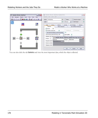
tbl[5,1][1,4] := "price";
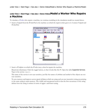
tbl[5,1][3,4] := "12,45";
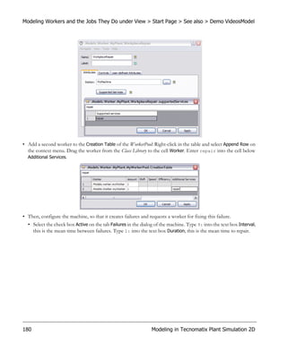
tbl[5,1][1,5] := "publish_date";
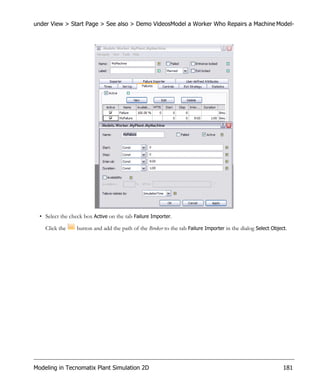
tbl[5,1][3,5] := "12.1.02";
tbl[5,1][1,6] := "description";
tbl[5,1][3,6] := "xx0011";
XMLInterface.insertNodes(tbl);
-- save the changed document
XMLInterface.filename := "D:MSXML 4.0tmp.xml";
XMLInterface.write;
-- close the document
XMLInterface.close;
end;
• Update the XML document.
-- updates the selected nodes of the document
is
tbl:table;
do
408 Importing Data for the Simulation](https://image.slidesharecdn.com/plantsimulationstep-by-stepenu-130104132843-phpapp02/85/Plant-Simulation-Passo-a-Passo-428-320.jpg)
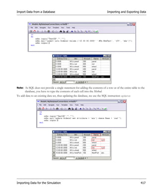
![Import Data in XML Format Importing and Exporting Data
XMLInterface.filename := "D:MSXML 4.0books.xml";
XMLInterface.openDocument;
-- select the nodes to be changed
tbl := XMLInterface.getNodes("/catalog/book[title='Midnight Rain']", 1);
-- update the values
tbl[5,1][3,3] := "TEST";
-- write the changed values
XMLInterface.updateNodes(tbl);
XMLInterface.filename := "D:MSXML 4.0tmp.xml";
XMLInterface.write;
XMLInterface.close;
end;
• Create a new XML document.
-- creates a new document by calling the method newDocument
is
tbl:table;
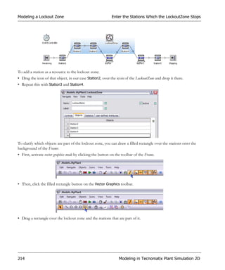
do
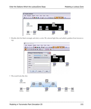
XMLInterface.newDocument("catalog");
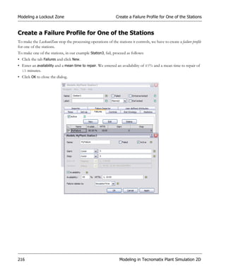
tbl := XMLInterface.getContainer(1);
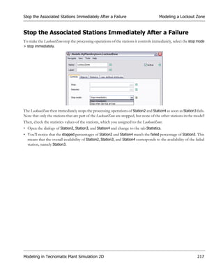
XMLInterface.setContext("/catalog");
-- parent node
tbl[1,1] := "book";
-- default namespace
tbl[2,1] := "MyBooks";
-- attributes
tbl.createNestedList(4,1);
-- explicit namespace
tbl[4,1][1,1] := "xmlns:aa";
tbl[4,1][2,1] := "specAth";
-- additional attributes
tbl[4,1][1,2] := "id";
tbl[4,1][2,2] := "bk113";
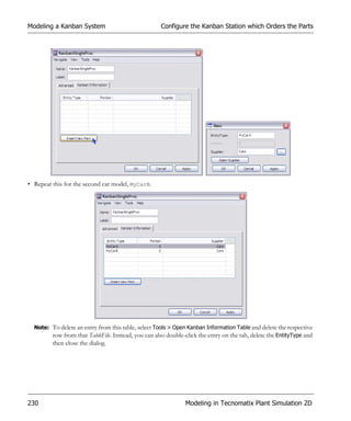
-- child nodes
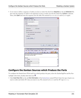
tbl.createNestedList(5,1);
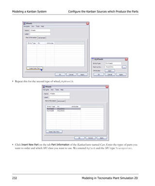
tbl[5,1][1,1] := "aa:author";
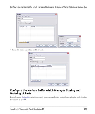
tbl[5,1][2,1] := "specAth";
tbl[5,1][3,1] := "XYZ";
tbl[5,1][1,2] := "title";
tbl[5,1][3,2] := "UNKNOWN";
tbl[5,1][1,3] := "genre";
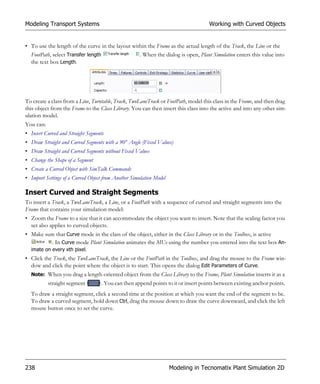
tbl[5,1][3,3] := "also";
tbl[5,1][1,4] := "price";
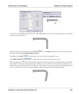
tbl[5,1][3,4] := "12,45";
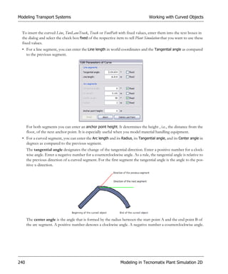
tbl[5,1][1,5] := "publish_date";
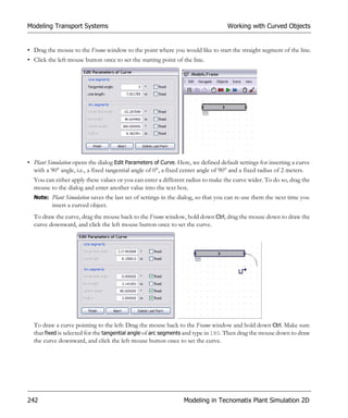
tbl[5,1][3,5] := "12.1.02";
Importing Data for the Simulation 409](https://image.slidesharecdn.com/plantsimulationstep-by-stepenu-130104132843-phpapp02/85/Plant-Simulation-Passo-a-Passo-429-320.jpg)
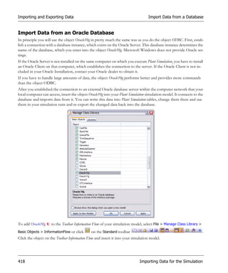
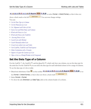
![Importing and Exporting Data Import Data from a Database
tbl[5,1][1,6] := "description";
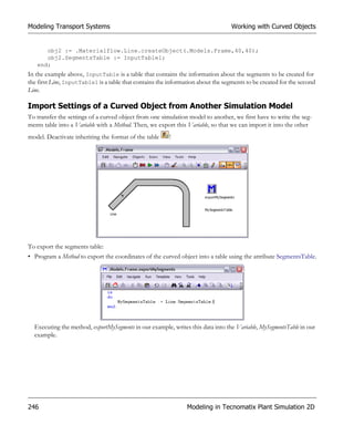
tbl[5,1][3,6] := "xx0011";
XMLInterface.insertNodes(tbl);
XMLInterface.filename := "D:MSXML 4.0tmp.xml";
XMLInterface.write;
end;
Access and Traverse Data Randomly
You can extract data in its entirety from an XML document and then randomly traverse the data. You might, for
example, define the starting point for traversing the structure with the method selectNodes. Then, you could get the
next node with the method getNodeName, check for attributes of this node with the method getNumberAttributes, out-
put the names of the attributes and recursively check all children of the selected node, to detect those that meet the
condition.
-- selects the starting nodes and calls the method visitChildren
-- recusively for each node
is
numberAttributes,i:integer;
do
XMLInterface.filename := "D:PublicXMLbooks.xml";
-- load the XML document to be randomly accessed into RAM
XMLInterface.openDocument;
-- select some nodes using XPath instructions
XMLInterface.selectNodes("book[genre = 'Computer']");
-- define the loop for the selected nodes
while XMLInterface.getNextNode = true loop
print XMLInterface.getNodeName;
-- check for attributes of the nodes
numberAttributes := XMLInterface.getNumberAttributes;
for i := 0 to numberAttributes-1 loop
-- print the data of the attributes
print XMLInterface.getAttributeName(i)+":"
+XMLInterface.getAttributeValue(i);
next;
-- check the children of the current node
VisitChildren;
end;
-- remove the XML document from RAM
XMLInterface.close;
end;
Import Data from a Database
You can import data from a database into Plant Simulation and run your simulation in Plant Simulation with this data.
You can then write the data resulting from the simulation runs back into the database.
410 Importing Data for the Simulation](https://image.slidesharecdn.com/plantsimulationstep-by-stepenu-130104132843-phpapp02/85/Plant-Simulation-Passo-a-Passo-430-320.jpg)
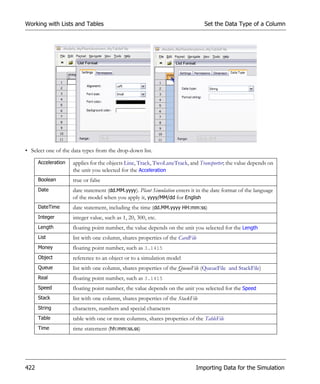
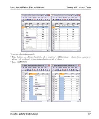
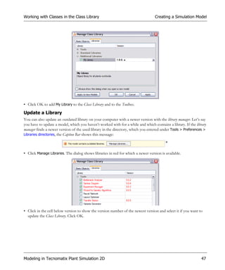
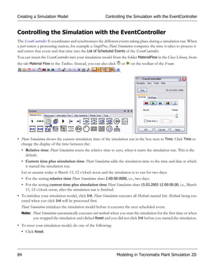
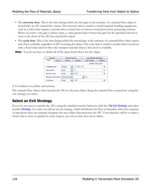
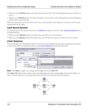
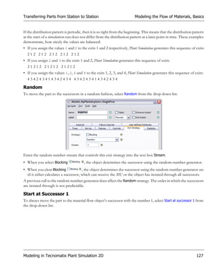
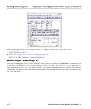
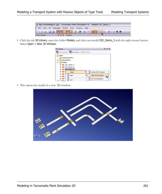
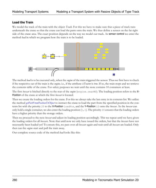
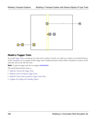
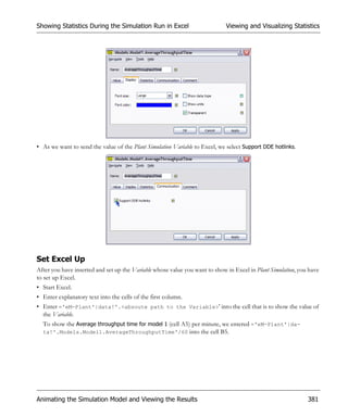
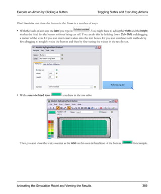
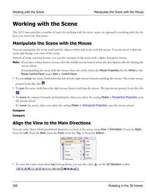
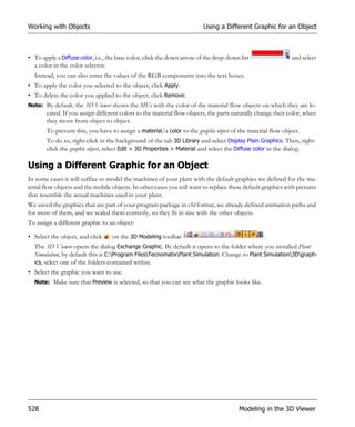
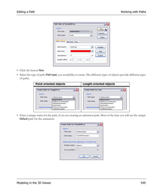
![Accessing Data in Lists Working with Lists and Tables
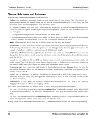
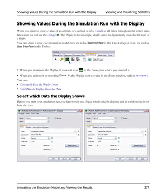
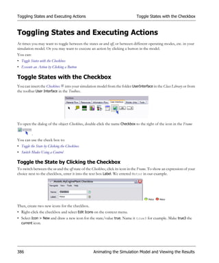
• Click the left mouse button and drag to the left until the columns you want to hide are not visible any more.
In the example we hid columns 2 through 14 . You recognize hidden columns by the symbol
that appears at the end of column 1.
To show hidden columns again, drag the cursor over the symbol. The cursor changes into an arrow pointing
to the right . To expand the columns to their original width, click the left mouse button once.
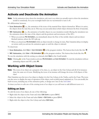
Accessing Data in Lists
To access a cell in a list or table with a Method, you can either use the system index, i.e., the number, which Plant
Simulation assigns to columns and rows or you can define your own user-defined index, which can be any mean-
ingful expression.
System index User-defined index
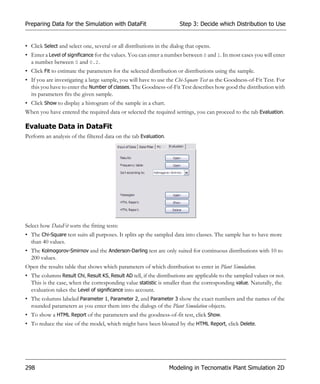
The advantage of a user-defined index over the standard system index is that assigning names to columns and rows
is more meaningful than the numbers, which Plant Simulation assigns by default. The user-defined index Vehi-
cles["Truck",#1] may tell you and your co-modelers more than the system index Vehicles[3,1] when de-
bugging your model. Both expressions access the same cell. As a user-defined index you might, for example, enter:
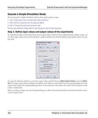
Switch["Light","220 Volts"];
Vehicles["Truck",#1];
Plant["Chicago",.building1.drill]
In addition, the user-defined index is not as error-prone as the system index: When you add an additional column
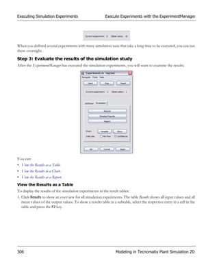
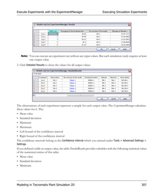
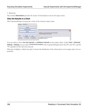
or a row to the table, Plant Simulation increases the system index of the succeeding columns or rows by one. This
naturally make any assignment in a Method to the previous system index invalid. The identifier of the user-defined
index, on the other hand, remains the same and is still valid. Be aware that accessing a user-defined index is slightly
slower than accessing the system index.
You can:
• Set the Column Index.
• Set the Row Index.
• Create a User-defined Column Index and a User-defined Row Index.
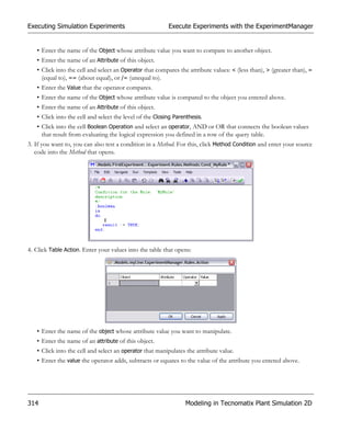
• Set and Get the Upper Bound of a List.
• Address Columns and Rows with Methods.
Importing Data for the Simulation 431](https://image.slidesharecdn.com/plantsimulationstep-by-stepenu-130104132843-phpapp02/85/Plant-Simulation-Passo-a-Passo-451-320.jpg)
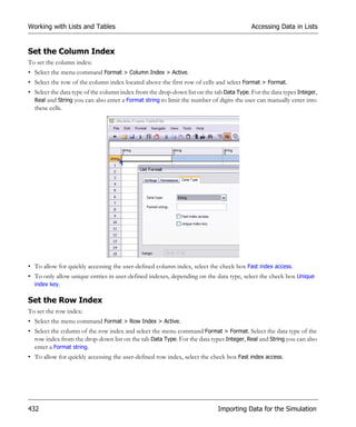
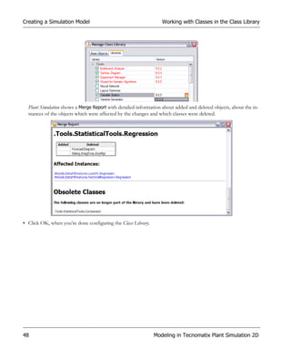
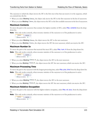
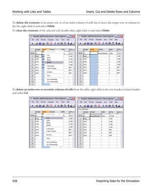
![Working with Lists and Tables Accessing Data in Lists
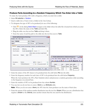
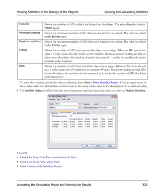
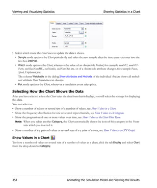
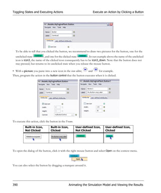
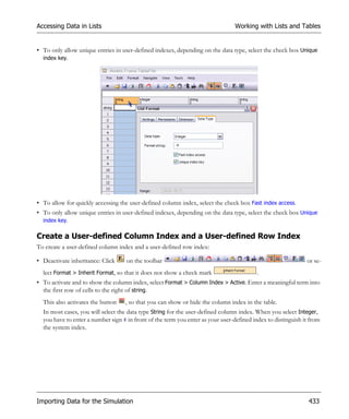
• To activate and to show the row index, select Format > Row Index > Active. Enter a meaningful expression into
the first column of cells below string 0.
This also activates the button , so that you can show or hide the row index in the table.
In most cases, you will select the data type String for the user-defined row index. When you select Integer, you
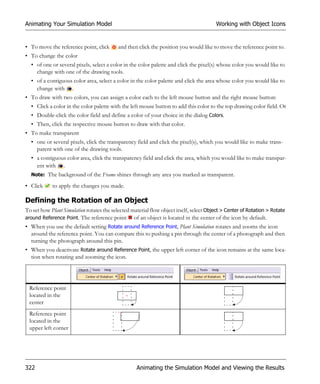
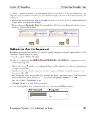
have to enter a number sign # in front of the expression, which you enter as your user-defined index, to distin-
guish it from the system index.
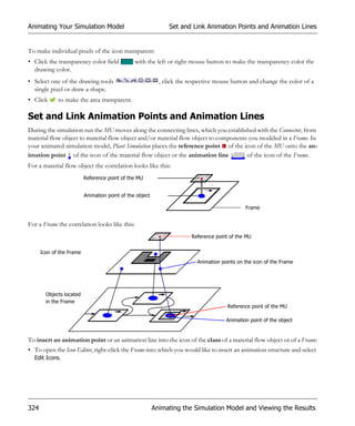
Note: When both column and row index are active, the cell [0,0], i.e., the cell at which column and row index in-
tersect, counts as part of the column index, not as part of the row index.
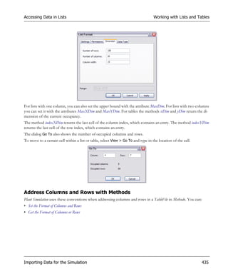
Set and Get the Upper Bound of a List
To set the upper bound of a list or table:
• Deactivate inheritance: Click on the toolbar or se-
lect Format > Inherit Format, so that it does not show a check mark .
• To select the entire list or table, click Select All or press Ctrl+A.
• Select Format > Format.
• Click the Tab Dimension. Enter the Number of columns and the Number of rows. Plant Simulation automatically
sets the lower bound to 1. When you use a user-defined index the lower bound is 0.
434 Importing Data for the Simulation](https://image.slidesharecdn.com/plantsimulationstep-by-stepenu-130104132843-phpapp02/85/Plant-Simulation-Passo-a-Passo-454-320.jpg)
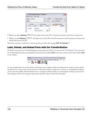
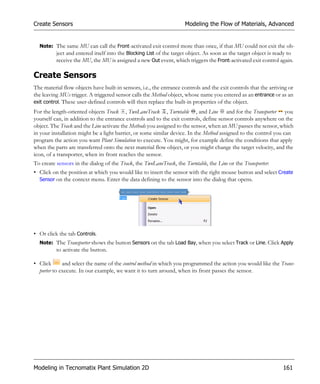
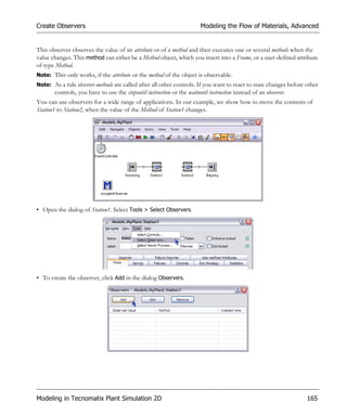
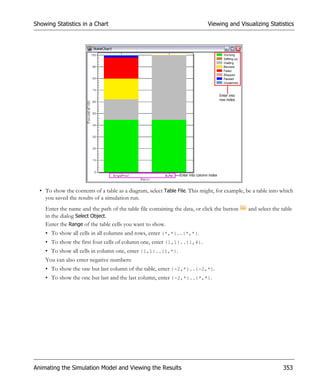
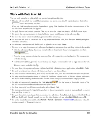
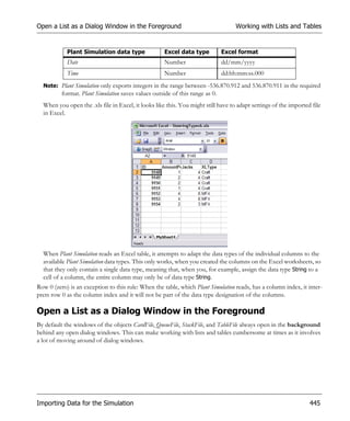
![Working with Lists and Tables Import or Export the Contents of a List
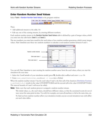
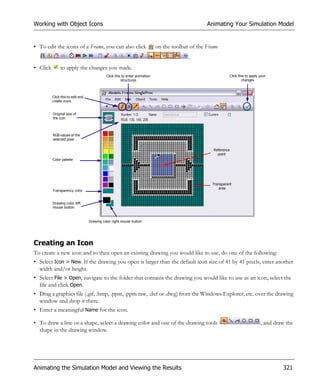
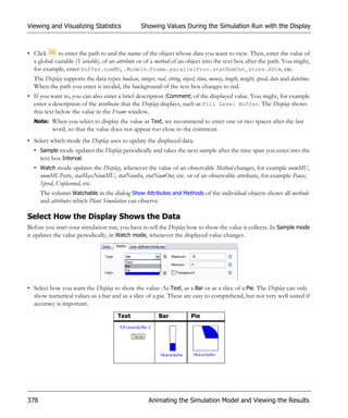
The list shows cells containing a formula in color. Turquoise designates a formula with a correct syntax, red a for-
mula with syntax errors.
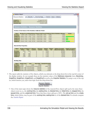
Within a formula you can access the value of another cell of the same list with the anonymous identifier @:
Formula Executes
@[1,1]+@[1,2] adds the contents of the cell [1,1] to the contents of the cell [1,2].
@[1,1]*track.length multiplies the contents of cell [1,1] with the length of the object track.
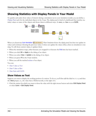
@[1,@.ydim]+5 adds 5 to the value of the last cell in the first column.
@[xSelf+1,ySelf]-7 subtracts 7 from the value of the neighboring cell to the right
@.sum({3,*}) calculates the sum of the third column.
@.min({1,2}..{1,*}) determines the smallest value of the first column, starting from cell 2.
Note: The data type of the result of a formula has to have the same data type as the cell or the column in which
the cell containing the formula is located.
In sublists, you can access the list, into which you inserted the sublist, with the anonymous identifier ?. Note that
for user-defined attributes of lists, the anonymous identifier ? accesses the object for which you defined the user-
defined attribute.
xSelf and ySelf contain the number of the column or the number of the row respectively, which contains the
formula. This way you can easily access neighboring cells.
Import or Export the Contents of a List
You can save an Plant Simulation list in several formats:
• To save the list with all of its Plant Simulation formatting as an Plant Simulation list, select File > Save As Object.
You can then open the saved list object within a list in other Frames or in other simulation models.
To import a TableFile, which you saved as an .obj file into another TableFile, select File > Open. To import a list
with one column into a TableFile, select the same data type for the left column that the list with one column has.
442 Importing Data for the Simulation](https://image.slidesharecdn.com/plantsimulationstep-by-stepenu-130104132843-phpapp02/85/Plant-Simulation-Passo-a-Passo-462-320.jpg)
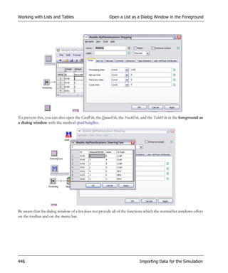
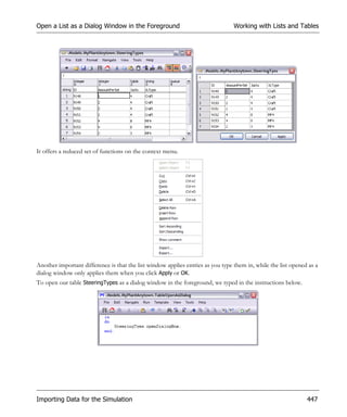
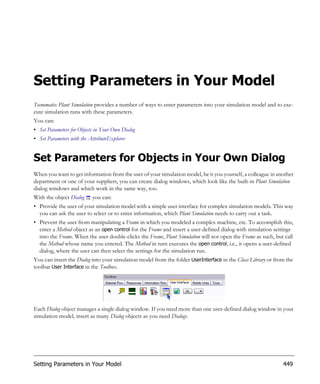
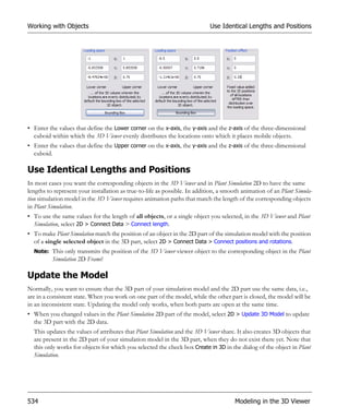


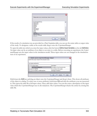
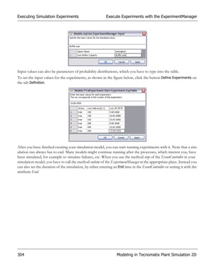
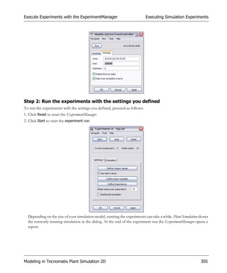
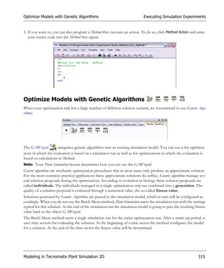
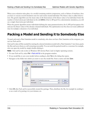
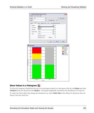
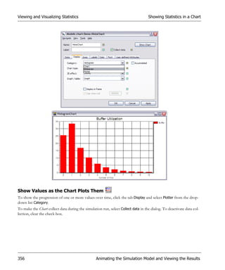
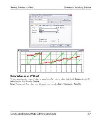
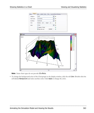
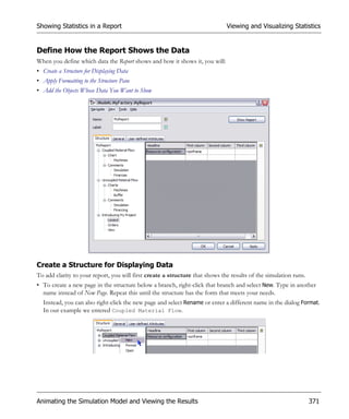
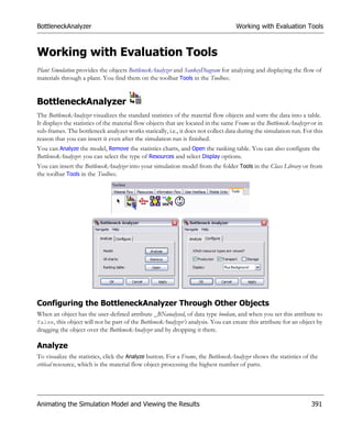
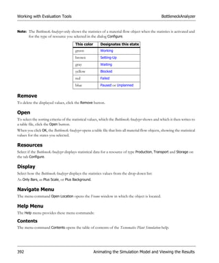
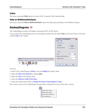
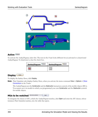
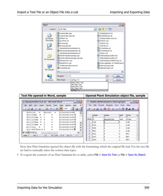
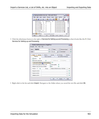
This document provides a proprietary step-by-step guide for the Technomatix Plant Simulation software version 10.1, including copyright and trademark information. It covers simulation concepts, implementation of simulation projects, and detailed instructions on using the program and its features. The document also includes tutorials, sample models, and explanation of classes and object management within the software.


![SCRM[1]](https://cdn.slidesharecdn.com/ss_thumbnails/6541d089-07f6-4578-95aa-2aba974be43e-151012061047-lva1-app6892-thumbnail.jpg?width=640&height=640&fit=bounds)