Downloaded 2,655 times


![1 Introduction
Scale Minimum and Maximum
The function premnmx can be used to scale inputs and targets so that they fall
in the range [-1,1].
Scale Mean and Standard Deviation
The function prestd normalizes the mean and standard deviation of the
training set.
Principal Component Analysis
The principle components analysis program prepca can be used to reduce the
dimensions of the input vectors.
Post-training Analysis
We have included a post training function postreg that performs a regression
analysis between the network response and the corresponding targets.
New Training Options
In this toolbox we can not only minimize mean squared error as before, but we
can also:
• Minimize with variations of mean squared error for better generalization.
Such training simplifies the problem of picking the number of hidden
neurons and produces good networks that are not overtrained.
• Train with validation to achieve appropriately early stopping. Here the
training result is checked against a validation set of input output data to
make sure that overtraining has not occurred.
• Stop training when the error gradient reaches a minimum. This avoids
wasting computation time when further training is having little effect.
• The low memory use Levenberg Marquardt algorithm has been incorporated
into both new and old algorithms.
1-10](https://image.slidesharecdn.com/nnet-090922002848-phpapp01/85/Neural-Network-Toolbox-MATLAB-30-320.jpg)
![1 Introduction
Neural Network Applications
The 1988 DARPA Neural Network Study [DARP88] lists various neural
network application, s beginning in about 1984 with the adaptive channel
equalizer. This device, which is an outstanding commercial success, is a single-
neuron network used in long distance telephone systems to stabilize voice
signals. The DARPA report goes on to list other commercial applications,
including a small word recognizer, a process monitor, a sonar classifier, and a
risk analysis system.
Neural networks have been applied in many other fields since the DARPA
report was written. A list of some applications mentioned in the literature
follows:
Aerospace
• High performance aircraft autopilot, flight path simulation, aircraft control
systems, autopilot enhancements, aircraft component simulation, aircraft
component fault detection
Automotive
• Automobile automatic guidance system, warranty activity analysis
Banking
• Check and other document reading, credit application evaluation
Defense
• Weapon steering, target tracking, object discrimination, facial recognition,
new kinds of sensors, sonar, radar and image signal processing including
data compression, feature extraction and noise suppression, signal/image
identification
Electronics
• Code sequence prediction, integrated circuit chip layout, process control,
chip failure analysis, machine vision, voice synthesis, nonlinear modeling
1-16](https://image.slidesharecdn.com/nnet-090922002848-phpapp01/85/Neural-Network-Toolbox-MATLAB-36-320.jpg)


![Data Structures
Data Structures
This section will discuss how the format of input data structures effects the
simulation of networks. We will begin with static networks and then move to
dynamic networks.
We will be concerned about two basic types of input vectors: those that occur
concurrently (at the same time, or in no particular time sequence) and those
that occur sequentially in time. For sequential vectors, the order in which the
vectors appear is important. For concurrent vectors, the order is not important,
and if we had a number of networks running in parallel we could present one
input vector to each of the networks.
Simulation With Concurrent Inputs in a Static
Network
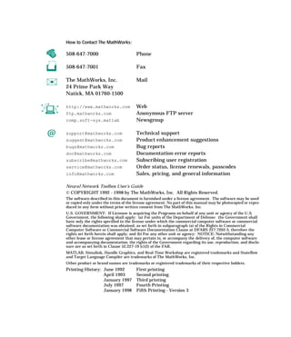
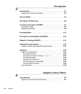
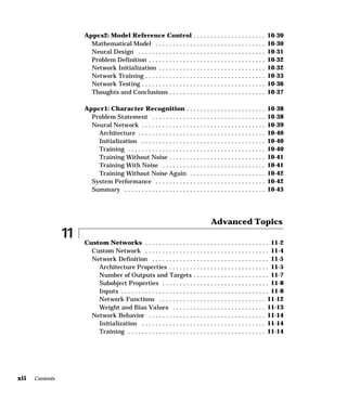
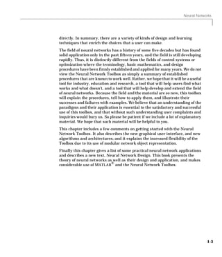
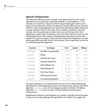
The simplest situation for simulating a network occurs when the network to be
simulated is static (has no feedback or delays). In this case we do not have to
be concerned about whether or not the input vectors occur in a particular time
sequence, so we can treat the inputs as concurrent. In addition, to make the
problem even simpler, we will begin by assuming that the network has only one
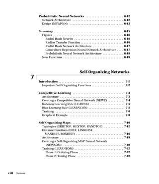
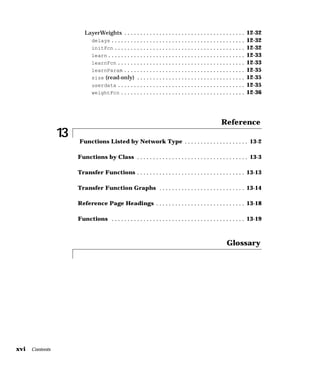
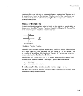
input vector. We will use the following network as an example.
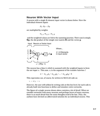
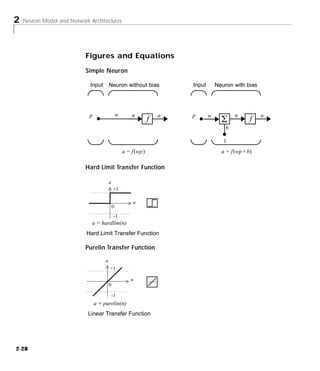
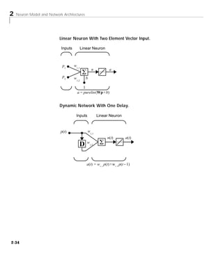
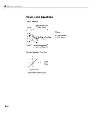
Inputs Linear Neuron
p1 w1,1
n a
p2 w1,2 b
1
a = purelin (Wp + b)
To set up this feedforward network we can use the following command.
net = newlin([-1 1;-1 1],1);
For simplicity we will assign the weight matrix and bias to be
W = 1 2 ,b = 0 .
2-15](https://image.slidesharecdn.com/nnet-090922002848-phpapp01/85/Neural-Network-Toolbox-MATLAB-55-320.jpg)
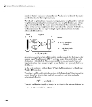
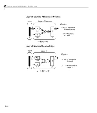
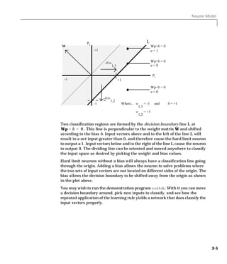
![2 Neuron Model and Network Architectures
The commands for these assignments are
net.IW{1,1} = [1 2];
net.b{1} = 0;
Suppose that the network simulation data set consists of Q = 4 concurrent
vectors:
p1 = 1 , p 2 = 2 , p 3 = 2 , p 4 = 3
2 1 3 1
Concurrent vectors are presented to the network as a single matrix:
P = [1 2 2 3; 2 1 3 1];
We can now simulate the network:
A = sim(net,P)
A =
5 4 8 5
A single matrix of concurrent vectors is presented to the network and the
network produces a single matrix of concurrent vectors as output. The result
would be the same if there were four networks operating in parallel and each
network received one of the input vectors and produced one of the outputs. The
ordering of the input vectors is not important as they do not interact with each
other.
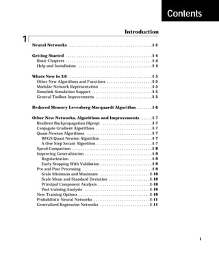
Simulation With Sequential Inputs in a Dynamic
Network
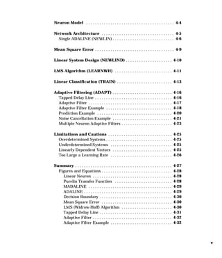
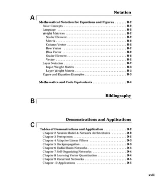
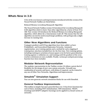
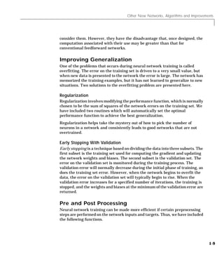
When a network contains delays, the input to the network would normally be
a sequence of input vectors which occur in a certain time order. To illustrate
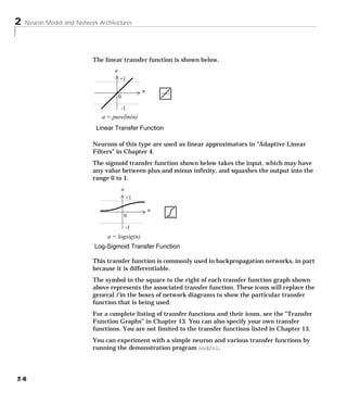
this case we will use a simple network which contains one delay.
2-16](https://image.slidesharecdn.com/nnet-090922002848-phpapp01/85/Neural-Network-Toolbox-MATLAB-56-320.jpg)
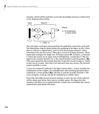
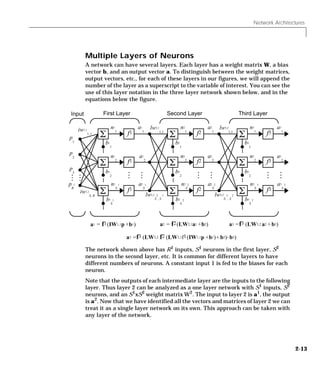
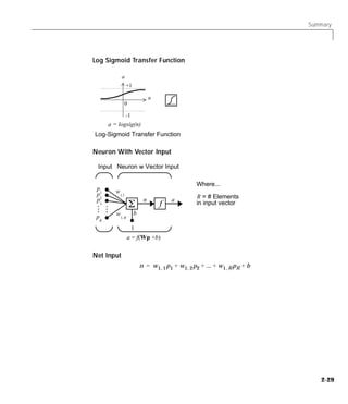
![Data Structures
Inputs Linear Neuron
p(t) w1,1
n(t) a(t)
w1,2
D
a(t) = w p(t) + w p(t - 1)
11 12
The following commands will create this network:
net = newlin([-1 1],1,[0 1]);
net.biasConnect = 0;
Assign the weight matrix to be
W = 1 2 .
The command is
net.IW{1,1} = [1 2];
Suppose that the input sequence is
p (1 ) = 1 , p( 2 ) = 2 , p ( 3 ) = 3 , p ( 4 ) = 4
Sequential inputs are presented to the network as elements of a cell array:
P = {1 2 3 4};
We can now simulate the network:
A = sim(net,P)
A =
[1] [4] [7] [10]
We input a cell array containing a sequence of inputs, and the network
produced a cell array containing a sequence of outputs. Note that the order of
the inputs is important when they are presented as a sequence. In this case the
current output is obtained by multiplying the current input by 1 and the
2-17](https://image.slidesharecdn.com/nnet-090922002848-phpapp01/85/Neural-Network-Toolbox-MATLAB-57-320.jpg)
![2 Neuron Model and Network Architectures
preceding input by 2 and summing the result. If we were to change the order of
the inputs it would change the numbers we would obtain in the output.
Simulation With Concurrent Inputs in a Dynamic
Network
If we were to apply the same inputs from the previous example as a set of
concurrent inputs instead of a sequence of inputs we would obtain a completely
different response. (Although it is not clear why we would want to do this with
a dynamic network.) It would be as if each input were applied concurrently to
a separate parallel network. For the previous example, if we use a concurrent
set of inputs we have
p1 = 1 , p 2 = 2 , p 3 = 3 , p 4 = 4 ,
which can be created with the following code:
P = [1 2 3 4];
When we simulate with concurrent inputs we obtain
A = sim(net,P)
A =
1 2 3 4
The result is the same as if we had concurrently applied each one of the inputs
to a separate network and computed one output. Note that since we did not
assign any initial conditions to the network delays they were assumed to be
zero. For this case the output will simply be 1 times the input, since the weight
which multiplies the current input is 1.
In certain special cases we might want to simulate the network response to
several different sequences at the same time. In this case we would want to
present the network with a concurrent set of sequences. For example, let’s say
we wanted to present the following two sequences to the network:
p1( 1 ) = 1 , p1( 2 ) = 2 , p1( 3 ) = 3 , p1(4 ) = 4 ,
p2( 1 ) = 4 , p2( 2 ) = 3 , p2( 3 ) = 2 , p2(4 ) = 1 .
The input P should be a cell array, where each element of the array contains
the two elements of the two sequences which occur at the same time:
P = {[1 4] [2 3] [3 2] [4 1]};
2-18](https://image.slidesharecdn.com/nnet-090922002848-phpapp01/85/Neural-Network-Toolbox-MATLAB-58-320.jpg)
![Data Structures
We can now simulate the network:
A = sim(net,P);
The resulting network output would be
A = {[ 1 4] [4 11] [7 8] [10 5]}
As you can see, the first column of each matrix makes up the output sequence
produced by the first input sequence, which was the one we used in an earlier
example. The second column of each matrix makes up the output sequence
produced by the second input sequence. There is no interaction between the
two concurrent sequences. It is as if they were each applied to separate
networks running in parallel.
The following diagram shows the general format for the input P to the sim
function when we have Q concurrent sequences of TS time steps. It covers all
cases where there is a single input vector. Each element of the cell array is a
matrix of concurrent vectors which correspond to the same point in time for
each sequence. If there are multiple input vectors there will be multiple rows
of matrices in the cell array.
Qth Sequence
·
{ [ p 1 ( 1 ), p 2 ( 1 ), …, p Q ( 1 ) ], [ p 1 ( 2 ), p 2 ( 2 ), …, p Q ( 2 ) ], …, [ p 1 ( TS ), p 2 ( TS ), …, p Q ( TS ) ] }
First Sequence
In this section we have applied sequential and concurrent inputs to dynamic
networks. In the previous section we applied concurrent inputs to static
networks. It is also possible to apply sequential inputs to static networks. It
will not change the simulated response of the network, but it can affect the way
in which the network is trained. This will become clear in the next section.
2-19](https://image.slidesharecdn.com/nnet-090922002848-phpapp01/85/Neural-Network-Toolbox-MATLAB-59-320.jpg)
![2 Neuron Model and Network Architectures
Training Styles
In this section we will describe two different styles of training. In incremental
training the weights and biases of the network are updated each time an input
is presented to the network. In batch training the weights and biases are only
updated after all of the inputs have been presented.
Incremental Training (of Adaptive and Other
Networks)
Incremental training can be applied to both static and dynamic networks,
although it is more commonly used with dynamic networks, such as adaptive
filters. In this section we will demonstrate how incremental training can be
performed on both static and dynamic networks.
Incremental Training with Static Networks
Consider again the static network we used for our first example. We want to
train it incrementally, so that the weights and biases will be updated after each
input is presented. In this case we use the function adapt, and we present the
inputs and targets as sequences.
Suppose we want to train the network to create the linear function
t = 2p 1 + p 2 .
Then for the previous inputs we used,
p1 = 1 , p 2 = 2 , p 3 = 2 , p 4 = 3 ,
2 1 3 1
the targets would be
t1 = 4 , t 2 = 5 , t 3 = 7 , t 4 = 7 .
We will first set up the network with zero initial weights and biases. We will
also set the learning rate to zero initially, in order to show the effect of the
incremental training.
net = newlin([-1 1;-1 1],1,0,0);
net.IW{1,1} = [0 0];
net.b{1} = 0;
2-20](https://image.slidesharecdn.com/nnet-090922002848-phpapp01/85/Neural-Network-Toolbox-MATLAB-60-320.jpg)
![Training Styles
For incremental training we want to present the inputs and targets as
sequences:
P = {[1;2] [2;1] [2;3] [3;1]};
T = {4 5 7 7};
Recall from the earlier discussion that for a static network the simulation of the
network will produce the same outputs whether the inputs are presented as a
matrix of concurrent vectors or as a cell array of sequential vectors. This is not
true when training the network, however. When using the adapt function, if
the inputs are presented as a cell array of sequential vectors, then the weights
will be updated as each input is presented (incremental mode). As we will see
in the next section, if the inputs are presented as a matrix of concurrent
vectors, then the weights will be updated only after all inputs have been
presented (batch mode).
We are now ready to train the network incrementally.
[net,a,e,pf] = adapt(net,P,T);
The network outputs will remain zero, since the learning rate is zero, and the
weights are not updated. The errors will be equal to the targets:
a = [0] [0] [0] [0]
e = [4] [5] [7] [7]
If we now set the learning rate to 0.1 we can see how the network is adjusted
as each input is presented:
net.inputWeights{1,1}.learnParam.lr=0.1;
net.biases{1,1}.learnParam.lr=0.1;
[net,a,e,pf] = adapt(net,P,T);
a = [0] [2] [6.0] [5.8]
e = [4] [3] [1.0] [1.2]
The first output is the same as it was with zero learning rate, since no update
is made until the first input is presented. The second output is different, since
the weights have been updated. The weights continue to be modified as each
error is computed. If the network is capable and the learning rate is set
correctly, the error will eventually be driven to zero.
2-21](https://image.slidesharecdn.com/nnet-090922002848-phpapp01/85/Neural-Network-Toolbox-MATLAB-61-320.jpg)
![2 Neuron Model and Network Architectures
Incremental Training With Dynamic Networks
We can also train dynamic networks incrementally. In fact, this would be the
most common situation. Let’s take the linear network with one delay at the
input that we used in a previous example. We will initialize the weights to zero
and set the learning rate to 0.1.
net = newlin([-1 1],1,[0 1],0.1);
net.IW{1,1} = [0 0];
net.biasConnect = 0;
To train this network incrementally we will present the inputs and targets as
elements of cell arrays.
Pi = {1};
P = {2 3 4};
T = {3 5 7};
Here we are attempting to train the network to sum the current and previous
inputs to create the current output. This is the same input sequence we used
in the previous example of using sim, except that we are assigning the first
term in the sequence as the initial condition for the delay. We are now ready to
sequentially train the network using adapt.
[net,a,e,pf] = adapt(net,P,T,Pi);
a = [0] [2.4] [ 7.98]
e = [3] [2.6] [-1.98]
The first output is zero, since the weights have not yet been updated. The
weights change at each subsequent time step.
Batch Training
Batch training, in which weights and biases are only updated after all of the
inputs and targets have been presented, can be applied to both static and
dynamic networks. We will discuss both types of networks in this section.
Batch Training With Static Networks
Batch training can be done using either adapt or train, although train is
generally the best option, since it typically has access to more efficient training
algorithms. Incremental training can only be done with adapt; train can only
perform batch training.
2-22](https://image.slidesharecdn.com/nnet-090922002848-phpapp01/85/Neural-Network-Toolbox-MATLAB-62-320.jpg)
![Training Styles
Let’s begin with the static network we used in previous examples. The learning
rate will be set to 0.1.
net = newlin([-1 1;-1 1],1,0,0.1);
net.IW{1,1} = [0 0];
net.b{1} = 0;
For batch training of a static network with adapt, the input vectors must be
placed in one matrix of concurrent vectors.
P = [1 2 2 3; 2 1 3 1];
T = [4 5 7 7];
When we call adapt it will invoke adaptwb, which is the default adaptation
function for the linear network, and learnwh is the default learning function
for the weights and biases. Therefore, Widrow-Hoff learning will be used.
[net,a,e,pf] = adapt(net,P,T);
a = 0 0 0 0
e = 4 5 7 7
Note that the outputs of the network are all zero, because the weights are not
updated until all of the training set has been presented. If we display the
weights we find:
»net.IW{1,1}
ans = 4.9000 4.1000
»net.b{1}
ans =
2.3000
This is different that the result we had after one pass of adapt with
incremental updating.
Now let’s perform the same batch training using train. Since the Widrow-Hoff
rule can be used in incremental or batch mode, it can be invoked by adapt or
train. There are several algorithms which can only be used in batch mode (e.g.,
Levenberg-Marquardt), and so these algorithms can only be invoked by train.
The network will be set up in the same way.
net = newlin([-1 1;-1 1],1,0,0.1);
net.IW{1,1} = [0 0];
net.b{1} = 0;
2-23](https://image.slidesharecdn.com/nnet-090922002848-phpapp01/85/Neural-Network-Toolbox-MATLAB-63-320.jpg)
![2 Neuron Model and Network Architectures
For this case the input vectors can either be placed in a matrix of concurrent
vectors or in a cell array of sequential vectors. Within train any cell array of
sequential vectors would be converted to a matrix of concurrent vectors. This
is because the network is static, and because train always operates in the
batch mode. Concurrent mode operation is generally used whenever possible,
because it has a more efficient MATLAB implementation.
P = [1 2 2 3; 2 1 3 1];
T = [4 5 7 7];
Now we are ready to train the network. We will train it for only one epoch, since
we used only one pass of adapt. The default training function for the linear
network is trainwb, and the default learning function for the weights and
biases is learnwh, so we should get the same results that we obtained using
adapt in the previous example, where the default adaptation function was
adaptwb.
net.inputWeights{1,1}.learnParam.lr = 0.1;
net.biases{1}.learnParam.lr = 0.1;
net.trainParam.epochs = 1;
net = train(net,P,T);
If we display the weights after one epoch of training we find:
»net.IW{1,1}
ans = 4.9000 4.1000
»net.b{1}
ans =
2.3000
This is the same result we had with the batch mode training in adapt. With
static networks the adapt function can implement incremental or batch
training depending on the format of the input data. If the data is presented as
a matrix of concurrent vectors batch training will occur. If the data is presented
as a sequence, incremental training will occur. This is not true for train, which
always performs batch training, regardless of the format of the input.
Batch Training With Dynamic Networks
Training static networks is relatively straightforward. If we use train the
network will be trained in the batch mode and the inputs will be converted to
concurrent vectors (columns of a matrix), even if they are originally passed as
a sequence (elements of a cell array). If we use adapt, the format of the input
2-24](https://image.slidesharecdn.com/nnet-090922002848-phpapp01/85/Neural-Network-Toolbox-MATLAB-64-320.jpg)
![Training Styles
will determine the method of training. If the inputs are passed as a sequence,
then the network will be trained in incremental mode. If the inputs are passed
as concurrent vectors, then batch mode training will be used.
With dynamic networks batch mode training would typically be done with
train only, especially if only one training sequence exists. To illustrate this,
let’s consider again the linear network with a delay. We will use a learning rate
of 0.02 for the training. (When using a gradient descent algorithm, we will
typically use a smaller learning rate for batch mode training than incremental
training, because all of the individual gradients are summed together before
determining the step change to the weights.)
net = newlin([-1 1],1,[0 1],0.02);
net.IW{1,1}=[0 0];
net.biasConnect=0;
net.trainParam.epochs = 1;
Pi = {1};
P = {2 3 4};
T = {3 5 6};
We want to train the network with the same sequence we used for the
incremental training earlier, but this time we want to update the weights only
after all of the inputs have been applied (batch mode). The network will be
simulated in sequential mode because the input is a sequence, but the weights
will be updated in batch mode.
net=train(net,P,T,Pi);
The weights after one epoch of training are
»net.IW{1,1}
ans = 0.9000 0.6200
These are different weights than we would obtain using incremental training,
where the weights would have been updated three times during one pass
through the training set. For batch training the weights are only updated once
in each epoch.
2-25](https://image.slidesharecdn.com/nnet-090922002848-phpapp01/85/Neural-Network-Toolbox-MATLAB-65-320.jpg)

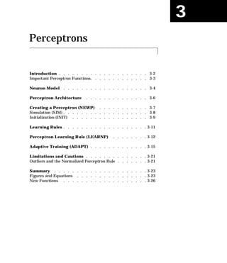
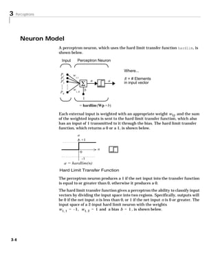
![3 Perceptrons
Introduction
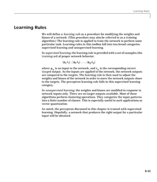
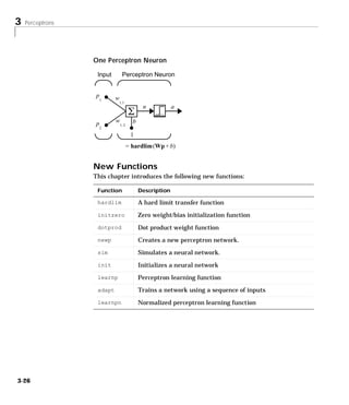
This chapter has a number of objectives. First we want to introduce you to
learning rules, methods of deriving the next changes that might be made in a
network, and training, a procedure whereby a network is actually adjusted to
do a particular job. Along the way we will discuss a toolbox function to create a
simple perceptron network, and we will also cover functions to initialize and
simulate such networks. We will use the perceptron as a vehicle for tying these
concepts together.
Rosenblatt [Rose61] created many variations of the perceptron. One of the
simplest was a single layer network whose weights and biases could be trained
to produce a correct target vector when presented with the corresponding input
vector. The training technique used is called the perceptron learning rule. The
perceptron generated great interest due to its ability to generalize from its
training vectors and learn from initially randomly distributed connections.
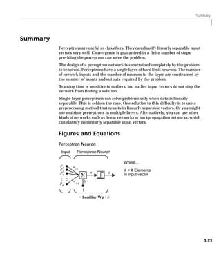
Perceptrons are especially suited for simple problems in pattern classification.
They are fast and reliable networks for the problems they can solve. In
addition, an understanding of the operations of the perceptron provides a good
basis for understanding more complex networks.
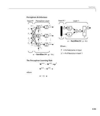
In this chapter we will define what we mean by a learning rule, explain the
perceptron network and its learning rule, and tell you how to initialize and
simulate perceptron networks.
The discussion of perceptron in this chapter is necessarily brief. You may wish
to read a more thorough discussion such as that given in Chapter 4 “Perceptron
Learning Rule,” of [HDB1996]. This Chapter discusses the use of multiple
layers of perceptrons to solve more difficult problems beyond the capability of
one layer.
You also may want to refer to the original book on the perceptron, Rosenblatt,
F., Principles of Neurodynamics, Washington D.C.: Spartan Press, 1961.
[Rose61].
3-2](https://image.slidesharecdn.com/nnet-090922002848-phpapp01/85/Neural-Network-Toolbox-MATLAB-76-320.jpg)
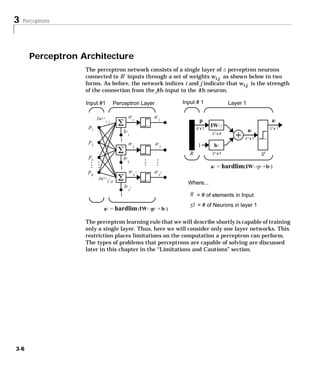
![Creating a Perceptron (NEWP)
Creating a Perceptron (NEWP)
A perceptron can be created with the function newp.
net = newp(PR, S)
where the input arguments are:
PR is an Rx2 matrix of minimum and maximum values for R input elements.
S is the Number of neurons.
Commonly the hardlim function is used in perceptrons, so it is the default.
The code below creates a peceptron network with a single one-element input
vector and one neuron. The range for the single element of the single input
vector is [0 2].
net = newp([0 2],1);
We can see what network has been created by executing the following code:
inputweights = net.inputweights{1,1}
which yields:
inputweights =
delays: 0
initFcn: 'initzero'
learn: 1
learnFcn: 'learnp'
learnParam: []
size: [1 1]
userdata: [1x1 struct]
weightFcn: 'dotprod'
Note that the default learning function is learnp, which will be discussed later
in this chapter. The net input to the hardlim transfer function is dotprod,
which generates the product of the input vector and weight matrix and adds
the bias to compute the net input.
Also note that the default initialization function, initzero, is used to set the
initial values of the weights to zero.
Similarly,
biases = net.biases{1}
3-7](https://image.slidesharecdn.com/nnet-090922002848-phpapp01/85/Neural-Network-Toolbox-MATLAB-81-320.jpg)
![3 Perceptrons
gives
biases =
initFcn: 'initzero'
learn: 1
learnFcn: 'learnp'
learnParam: []
size: 1
userdata: [1x1 struct].
We can see that the default initialization for the bias is also 0.
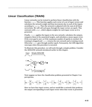
Simulation (SIM)
To show how sim works we will examine a simple problem.
Suppose we take a perceptron with a single two element input vector, like that
discussed in the decision boundary figure. We define the network with:
net = newp([-2 2;-2 +2],1);
As noted above, this will give us zero weights and biases, so if we want a
particular set other than zeros, we will have to create them. We can set the two
weights and the one bias to -1, 1 and 1 as they were in the decision boundary
figure with the following two lines of code.
net.IW{1,1}= [-1 1];
net.b{1} = [1];
To make sure that these parameters were set correctly, we will check them
with:
net.IW{1,1}
ans =
-1 1
net.b{1}
ans =
1
3-8](https://image.slidesharecdn.com/nnet-090922002848-phpapp01/85/Neural-Network-Toolbox-MATLAB-82-320.jpg)
![Creating a Perceptron (NEWP)
Now let us see if the network responds to two signals, one on each side of the
perceptron boundary.
p1 = [1;1];
a1 = sim(net,p1)
a1 =
1
and for
p2 = [1;-1]
a2 = sim(net,p2)
a2 =
0
Sure enough, the perceptron has classified the two inputs correctly.
Note that we could have presented the two inputs in a sequence and gotten the
outputs in a sequence as well.
p3 = {[1;1] [1;-1]};
a3 = sim(net,p3)
a3 =
[1] [0]
Initialization (INIT)
You can use the function init to reset the network weights and biases to their
original values. Suppose, for instance that you start with the network:
net = newp([-2 2;-2 +2],1);
Now check its weights with
wts = net.IW{1,1}
which gives, as expected,
wts =
0 0
In the same way, you can verify that the bias is 0 with
bias = net.b{1}
3-9](https://image.slidesharecdn.com/nnet-090922002848-phpapp01/85/Neural-Network-Toolbox-MATLAB-83-320.jpg)
![3 Perceptrons
which gives
bias =
0.
Now set the weights to the values 3 and 4 and the bias to the value 5 with
net.IW{1,1} = [3,4];
net.b{1} = 5;
Recheck the weights and bias as shown above to verify that the change has
been made. Sure enough,
wts =
3 4
bias =
5.
Now use init to reset the weights and bias to their original values.
net = init(net);
We can check as shown above to verify that:
wts =
0 0
bias =
0.
We can change the as way that a perceptron is initialized with init. For
instance, suppose that we define the network input weights and bias initFcns
as rands and then apply init as shown below.
net.inputweights{1,1}.initFcn = 'rands';
net.biases{1}.initFcn = 'rands';
net = init(net);
Now check on the weights and bias.
wts =
0.2309 0.5839
biases =
-0.1106
We can see that the weights and bias have been given random numbers.
3-10](https://image.slidesharecdn.com/nnet-090922002848-phpapp01/85/Neural-Network-Toolbox-MATLAB-84-320.jpg)
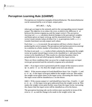
![Perceptron Learning Rule (LEARNP)
CASE 1. If e = 0, then make a change ∆w equal to 0.
CASE 2. If e = 1, then make a change ∆w equal to pT.
CASE 3. If e = –1, then make a change ∆w equal to –pT.
All three cases can then be written with a single expression:
∆w = ( t – a )p T = ep T
We can get the expression for changes in a neuron’s bias by noting that the bias
is simply a weight which always has an input of 1:
∆b = ( t – a ) ( 1 ) = e
For the case of a layer of neurons we have:
∆W = ( t – a ) ( p ) T = e ( p ) T and
∆b = ( t – a ) = E
The Perceptron Learning Rule can be summarized as follows:
new old T
W = W + ep and
ne w o ld
b = b +e
where e = t – a .
Now let us try a simple example. We will start with a single neuron having a
input vector with just two elements.
net = newp([-2 2;-2 +2],1);
To simplify matters we will set the bias equal to 0 and the weights to 1 and -0.8.
net.biases{1}.value = [0];
w = [1 -0.8];
net.IW{1,1}.value = w;
The input target pair is given by:
p = [1; 2];
t = [1];
3-13](https://image.slidesharecdn.com/nnet-090922002848-phpapp01/85/Neural-Network-Toolbox-MATLAB-87-320.jpg)
![3 Perceptrons
We can compute the output and error with
a = sim(net,p)
a =
0
e = t-a
e =
1
and finally use the function learnp to find the change in the weights.
dw = learnp(w,p,[],[],[],[],e,[],[],[])
dw =
1 2.
The new weights, then, are obtained as
w = w + dw
w =
2.0000 1.2000
The process of finding new weights (and biases) can be repeated until there are
no errors. Note that the perceptron learning rule is guaranteed to converge in
a finite number of steps for all problems that can be solved by a perceptron.
These include all classification problems that are “linearly separable.” The
objects to be classified in such cases can be separated by a single line.
You might want to try demo nnd4pr. It allows you to pick new input vectors and
apply the learning rule to classify them.
3-14](https://image.slidesharecdn.com/nnet-090922002848-phpapp01/85/Neural-Network-Toolbox-MATLAB-88-320.jpg)
![Adaptive Training (ADAPT)
Adaptive Training (ADAPT)
If sim and learnp are used repeatedly to present inputs to a perceptron, and to
change the perceptron weights and biases according to the error, the
perceptron will eventually find weight and bias values which solve the
problem, given that the perceptron can solve it. Each traverse through all of the
training input and target vectors is called a pass.
The function adapt carries out such a loop of calculation. In each pass the
function adapt will proceed through the specified sequence of inputs,
calculating the output, error and network adjustment for each input vector in
the sequence as the inputs are presented.
Note that adapt does not guarantee that the resulting network does its job.
The new values of W and b must be checked by computing the network output
for each input vector to see if all targets are reached. If a network does not
perform successfully it can be trained further by again calling adapt with the
new weights and biases for more training passes, or the problem can be
analyzed to see if it is a suitable problem for the perceptron. Problems which
are not solvable by the perceptron network are discussed in the “Limitations
and Cautions” section.
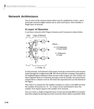
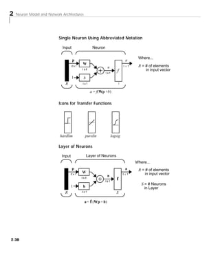
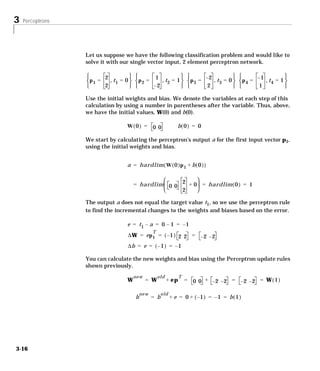
To illustrate the adaptation procedure, we will work through a simple problem.
Consider a one neuron perceptron with a single vector input having two
elements.
Input Perceptron Neuron
p w
1
1,1
n a
f
p w b
1, 2
2
1
a = hardlim-(Wp + b)
- Exp
This network, and the problem we are about to consider are simple enough that
you can follow through what is done with hand calculations if you wish. The
problem discussed below follows that found in [HDB1996].
3-15](https://image.slidesharecdn.com/nnet-090922002848-phpapp01/85/Neural-Network-Toolbox-MATLAB-89-320.jpg)
![Adaptive Training (ADAPT)
Now present the next input vector, p2. The output is calculated below.
a = hardlim ( W ( 1 )p 2 + b ( 1 ) )
= hardlim – 2 – 2 – 2 – 1 = hardlim ( 1 ) = 1
–2
On this occasion, the target is 1, so the error is zero. Thus there are no changes
in weights or bias so W ( 2 ) = W ( 1 ) = – 2 – 2 and p ( 2 ) = p ( 1 ) = – 1
We can continue in this fashion, presenting p3 next, calculating an output and
the error, and making changes in the weights and bias, etc. After making one
pass through all of the four inputs, you will get the values: W ( 4 ) = – 3 – 1
and b ( 4 ) = 0 . To determine if we have obtained a satisfactory solution, we
must make one pass through all input vectors to see if they all produce the
desired target values. This is not true for the 4th input, but the algorithm does
converge on the 6th presentation of an input. The final values are:
W ( 6 ) = – 2 – 3 and b ( 6 ) = 1 .
This concludes our hand calculation. Now, how can we do this using the adapt
function?
The following code defines a perceptron like that shown in the previous figure,
with initial weights and bias values of 0.
net = newp([-2 2;-2 +2],1);
Let us first consider the application of a single input. We will define the first
input vector and target as sequences (cell arrays in curly brackets).
p = {[2; 2]};
t = {0}
Now set passes to 1, so that adapt will go through the input vectors (only one
here) just one time.
net.adaptParam.passes = 1;
[net,a,e] = adapt(net,p,t);
3-17](https://image.slidesharecdn.com/nnet-090922002848-phpapp01/85/Neural-Network-Toolbox-MATLAB-91-320.jpg)
![3 Perceptrons
The output and error that are returned are:
a =
[1]
e =
[-1]
The new weights and bias are:
twts = net.IW{1,1}
twts =
-2 -2
tbiase = net.b{1}
tbiase =
-1
Thus, the initial weights and bias are 0, and after training on just the first
vector they have the values [-2 -2] and -1, just as we hand calculated.
We now apply the second input vector p 2 . The output is 1, as it will be until the
weights and bias are changed, but now the target is 1, the error will be 0 and
the change will be zero. We could proceed in this way, starting from the
previous result and applying a new input vector time after time. But we can do
this job automatically with adapt.
Now let’s apply adapt for one pass through the sequence of all four input
vectors. Start with the network definition.
net = newp([-2 2;-2 +2],1);
net.trainParam.passes = 1;
The input vectors and targets are:
p = {[2;2] [1;-2] [-2;2] [-1;1]}
t = {0 1 0 1}.
Now train the network with:
[net,a,e] = adapt(net,p,t);
3-18](https://image.slidesharecdn.com/nnet-090922002848-phpapp01/85/Neural-Network-Toolbox-MATLAB-92-320.jpg)
![Adaptive Training (ADAPT)
The output and error that are returned are:
a =
[1] [1] [0] [0]
e =
[-1] [0] [0] [1]
Note that these outputs and errors are the values obtained when each input
vector is applied to the network as it existed at the time.
The new weights and bias are:
twts =
-3 -1
tbias =
0
Finally simulate the trained network for each of the inputs.
a1 = sim(net,p)
a1 =
[0] [0] [1] [1]
The outputs do not yet equal the targets, so we need to train the network for
more than one pass. This time let us run the problem again for two passes. We
get the weights
twts =
-2 -3
tbiase =
1
and the simulated output and errors for the various inputs is:
a1 =
[0] [1] [0] [1]
The second pass does the job. The network has converged and produces the
correct outputs for the four input vectors. To check we can find the error for
each of the inputs.
error = {a1{1}-t{1} a1{2}-t{2} a1{3}-t{3} a1{4}-t{4}}
error =
[0] [0] [0] [0]
Sure enough, all of the inputs are correctly classified.
3-19](https://image.slidesharecdn.com/nnet-090922002848-phpapp01/85/Neural-Network-Toolbox-MATLAB-93-320.jpg)

![Limitations and Cautions
Limitations and Cautions
Perceptron networks should be trained with adapt, which presents the input
vectors to the network one at a time and makes corrections to the network
based on the results of each presentation. Use of adapt in this way guarantees
that any linearly separable problem will be solved in a finite number of
training presentations. Perceptrons can also be trained with the function
train, which is presented in the next chapter. When train is used for
perceptrons, it presents the inputs to the network in batches, and makes
corrections to the network based on the sum of all the individual corrections.
Unfortunately, there is no proof that such a training algorithm converges for
perceptrons. On that account the use of train for perceptrons is not
recommended.
Perceptron networks have several limitations. First, the output values of a
perceptron can take on only one of two values (0 or 1) due to the hard limit
transfer function. Second, perceptrons can only classify linearly separable sets
of vectors. If a straight line or a plane can be drawn to separate the input
vectors into their correct categories, the input vectors are linearly separable. If
the vectors are not linearly separable, learning will never reach a point where
all vectors are classified properly. Note, however, that it has been proven that
if the vectors are linearly separable, perceptrons trained adaptively will always
find a solution in finite time. You might want to try demop6. It shows the
difficulty of trying to classify input vectors that are not linearly separable.
It is only fair, however, to point out that networks with more than one
perceptron can be used to solve more difficult problems. For instance, suppose
that you have a set of four vectors that you would like to classify into distinct
groups, and that in fact, two lines can be drawn to separate them. A two neuron
network can be found such that its two decision boundaries classify the inputs
into four categories. For additional discussion about perceptrons and to
examine more complex perceptron problems, see [HDB1996].
Outliers and the Normalized Perceptron Rule
Long training times can be caused by the presence of an outlier input vector
whose length is much larger or smaller than the other input vectors. Applying
the perceptron learning rule involves adding and subtracting input vectors
from the current weights and biases in response to error. Thus, an input vector
with large elements can lead to changes in the weights and biases that take a
3-21](https://image.slidesharecdn.com/nnet-090922002848-phpapp01/85/Neural-Network-Toolbox-MATLAB-95-320.jpg)
![4 Adaptive Linear Filters
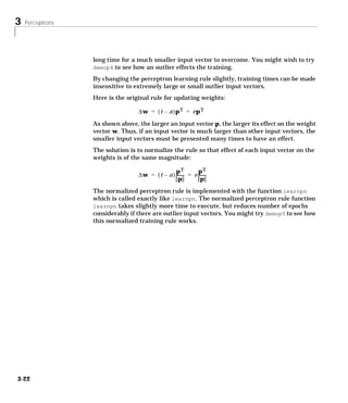
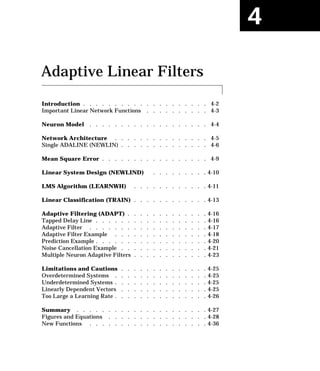
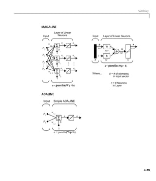
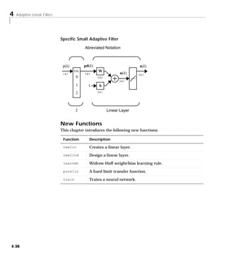
Single ADALINE (NEWLIN)
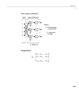
Consider a single ADALINE with two inputs. The diagram for this network is
shown below.
Input Simple ADALINE
p1 w
1,1
n a
p2 w1,2 b
1
a = purelin(Wp+b)
The weight matrix W in this case has only one row. The network output is:
a = purelin ( n ) = purelin ( Wp + b ) = Wp + b or
a = w 1, 1 p 1 + w 1, 2 p 2 + b
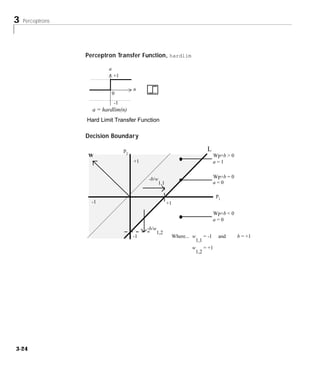
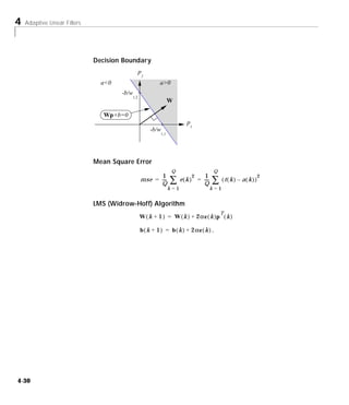
Like the perceptron, the ADALINE has a decision boundary which is
determined by the input vectors for which the net input n is zero. For n = 0
the equation Wp + b = 0 specifies such a decision boundary as shown below
(adapted with thanks from [HDB96]).
p
2
a<0 a>0
-b/w
1,2
W
Wp+b=0
p
1
-b/w
1,1
Input vectors in the upper right gray area will lead to an output greater than
0. Input vectors in the lower left white area will lead to an output less than 0.
Thus, the ADALINE can be used to classify objects into two categories.
4-6](https://image.slidesharecdn.com/nnet-090922002848-phpapp01/85/Neural-Network-Toolbox-MATLAB-106-320.jpg)
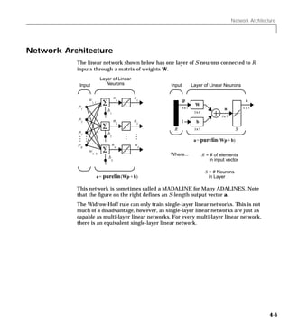
![Network Architecture
However, it can classify in this way only if the objects are linearly separable.
Thus, the ADALINE has the same limitation as the perceptron.
We can create a network like that shown above with the command:
net = newlin( [-1 1; -1 1],1);
The first matrix of arguments specify the range of the two scalar inputs. The
last argument, 1, says that the network has a single output.
The network weights and biases are set to zero by default. You can see the
current values with the commands:
W = net.IW{1,1}
W =
0 0
and
b= net.b{1}
b =
0
However, you can give the weights any value that you wish, such as 2 and 3
respectively, with:
net.IW{1,1} = [2 3];
W = net.IW{1,1}
W =
2 3
The bias can be set and checked in the same way.
net.b{1} =[-4];
b = net.b{1}
b =
-4
You can simulate the ADALINE for a particular input vector. Let us try
p = [5;6];
4-7](https://image.slidesharecdn.com/nnet-090922002848-phpapp01/85/Neural-Network-Toolbox-MATLAB-107-320.jpg)

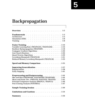
![Mean Square Error
Mean Square Error
Like the perceptron learning rule, the least mean square error (LMS)
algorithm is an example of supervised training, in which the learning rule is
provided with a set of examples of desired network behavior:
{p 1, t 1} , { p2, t 2} , …, {p Q, tQ}
Here pq is an input to the network, and t q is the corresponding target output.
As each input is applied to the network, the network output is compared to the
target. The error is calculated as the difference between the target output and
the network output. We want to minimize the average of the sum of these
errors.
Q Q
∑ ∑
1 2 1 2
mse = ---
- e ( k ) = ---
- (t( k ) – a( k ) )
Q Q
k=1 k=1
The LMS algorithm adjusts the weights and biases of the ADALINE so as to
minimize this mean square error.
Fortunately, the mean square error performance index for the ADALINE
network is a quadratic function. Thus, the performance index will either have
one global minimum, a weak minimum or no minimum, depending on the
characteristics of the input vectors. Specifically, the characteristics of the
input vectors determine whether or not a unique solution exists.
You can find more about this topic in Ch. 10 of [HDB96].
4-9](https://image.slidesharecdn.com/nnet-090922002848-phpapp01/85/Neural-Network-Toolbox-MATLAB-109-320.jpg)
![4 Adaptive Linear Filters
Linear System Design (NEWLIND)
Unlike most other network architectures, linear networks can be designed
directly if all input/target vector pairs are known. Specific network values for
weights and biases can be obtained to minimize the mean square error by using
the function newlind.
Suppose that the inputs and targets are:
P = [1 2 3];
T= [2.0 4.1 5.9];
Now you can design a network.
net = newlind(P,T);
You can simulate the network behavior to check that the design was done
properly.
Y = sim(net,P)
Y =
2.0500 4.0000 5.9500
Note that the network outputs are quite close to the desired targets.
You might try demolin1. It shows error surfaces for a particular problem,
illustrates the design and plots the designed solution.
Next we will discuss the LMS algorithm. We can use it to train a network to
minimize the mean square error.
4-10](https://image.slidesharecdn.com/nnet-090922002848-phpapp01/85/Neural-Network-Toolbox-MATLAB-110-320.jpg)
![LMS Algorithm (LEARNWH)
LMS Algorithm (LEARNWH)
The LMS algorithm or Widrow-Hoff learning algorithm, is based on an
approximate steepest descent procedure. Here again, linear networks are
trained on examples of correct behavior.
Widrow and Hoff had the insight that they could estimate the mean square
error by using the squared error at each iteration. If we take the partial
derivative of the squared error with respect to the weights and biases at the kth
iteration we have:
2
∂e ( k ) ∂e ( k )
---------------- = 2e ( k ) -------------
- -
∂w 1, j ∂w 1, j
for j = 1, 2, …, R and
2
∂e ( k ) ∂e ( k )
---------------- = 2e ( k ) -------------
- -
∂b ∂b
Next look at the partial derivative with respect to the error.
∂e ( k ) ∂[ t ( k ) – a ( k ) ] ∂
------------- = ----------------------------------- =
- - [ t ( k ) – ( Wp ( k ) + b ) ] or
∂w 1, j ∂w 1, j ∂ w 1, j
R
∂e ( k ) ∂
------------- =
∂w 1, j
-
∂ w 1, j
t(k) – ∑
i=1
w 1, i p i ( k ) + b
Here pi(k) is the ith element of the input vector at the kth iteration.
Similarly,
∂e ( k )
------------- = – p j ( k )
-
∂w 1, j
This can be simplified to:
∂e ( k )
------------- = – p j ( k ) and
-
∂w 1, j
∂e ( k )
------------- = – 1
-
∂b
4-11](https://image.slidesharecdn.com/nnet-090922002848-phpapp01/85/Neural-Network-Toolbox-MATLAB-111-320.jpg)
![4 Adaptive Linear Filters
Finally, the change to the weight matrix and the bias will be:
2αe ( k )p ( k ) and 2αe ( k ) . These two equations form the basis of the
Widrow-Hoff (LMS) learning algorithm.
These results can be extended to the case of multiple neurons, and written in
matrix form as:
T
W ( k + 1 ) = W ( k ) + 2αe ( k )p ( k )
b ( k + 1 ) = b ( k ) + 2αe ( k ) .
Here the error e and the bias b are vectors and α is a learning rate. If α is
large, learning occurs quickly, but if it is too large it may lead to instability and
errors may even increase. To ensure stable learning, the learning rate must be
less than the reciprocal of the largest eigenvector of the correlation matrix
p T p of the input vectors.
You might want to read some of Chapter 10 of [HDB96] for more information
about the LMS algorithm and its convergence.
Fortunately we have a toolbox function learnwh that does all of the calculation
for us. It calculates the change in weights as
dw = lr*e*p'
and the bias change as
db = lr*e.
The constant 2 shown a few lines above has been absorbed into the code
learning rate lr. The function maxlinlr calculates this maximum stable
learning rate lr as 0.999 * P'*P.
Type help learnwh and help maxlinlr for more details about these two
functions.
4-12](https://image.slidesharecdn.com/nnet-090922002848-phpapp01/85/Neural-Network-Toolbox-MATLAB-112-320.jpg)
![4 Adaptive Linear Filters
We will use train to get the weights and biases for a network that produces
the correct targets for each input vector. The initial weights and bias for the
new network will be 0 by default. We will set the error goal to 0.1 rather than
accept its default of 0.
P = [2 1 -2 -1;2 -2 2 1];
t = [0 1 0 1];
net = newlin( [-2 2; -2 2],1);
net.trainParam.goal= 0.1;
[net, tr] = train(net,P,t);
The problem runs, producing the following training record.
TRAINWB, Epoch 0/100, MSE 0.5/0.1.
TRAINWB, Epoch 25/100, MSE 0.181122/0.1.
TRAINWB, Epoch 50/100, MSE 0.111233/0.1.
TRAINWB, Epoch 64/100, MSE 0.0999066/0.1.
TRAINWB, Performance goal met.
Thus, the performance goal is met in 64 epochs. The new weights and bias are:
weights = net.iw{1,1}
weights =
-0.0615 -0.2194
bias = net.b(1)
bias =
[0.5899]
We can simulate the new network as shown below.
A = sim(net, p)
A =
0.0282 0.9672 0.2741 0.4320,
We also can calculate the error.
err = t - sim(net,P)
err =
-0.0282 0.0328 -0.2741 0.5680
Note that the targets are not realized exactly. The problem would have run
longer in an attempt to get perfect results had we chosen a smaller error goal,
but in this problem it is not possible to obtain a goal of 0. The network is limited
4-14](https://image.slidesharecdn.com/nnet-090922002848-phpapp01/85/Neural-Network-Toolbox-MATLAB-114-320.jpg)

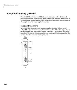
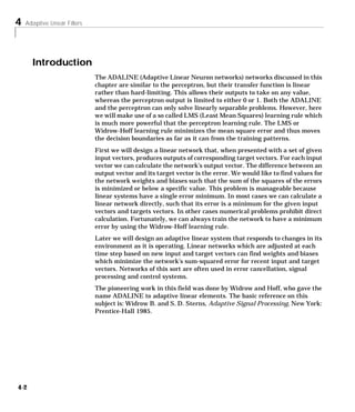
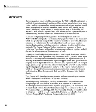
![Adaptive Filtering (ADAPT)
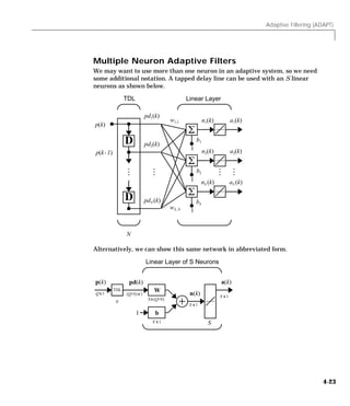
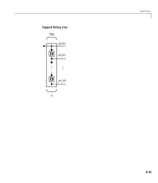
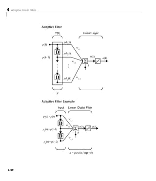
Adaptive Filter
We can combine a tapped delay line with an ADALINE network to create the
adaptive filter shown below.
TDL Linear Layer
pd (k)
1
p(k)
w
1,1
D pd (k)
2
p(k - 1) n(k)
a(k)
SxR
w1,2
b
1
D pdN (k) w1, N
N
The output of the filter is given by
R
a ( k ) = purelin ( Wp + b ) = ∑ w 1, i a ( k – i + 1 ) + b
i=1
The network shown above is referred to in the digital signal processing field as
a finite impulse response (FIR) filter [WiSt85]. Let us take a look at the code
that we will use to generate and simulate such an adaptive network.
4-17](https://image.slidesharecdn.com/nnet-090922002848-phpapp01/85/Neural-Network-Toolbox-MATLAB-117-320.jpg)
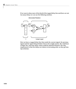
![4 Adaptive Linear Filters
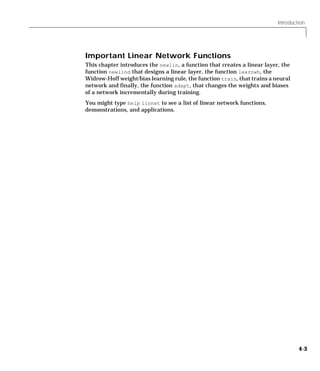
Adaptive Filter Example
First we will define a new linear network using newlin.
Input Linear Digital Filter
p (t) = p(t)
1
w1,1
D w1,2
n(t) a(t)
p (t) = p(t - 1)
2
b
D w
1,3
1
p3(t) = p(t - 2)
- Exp -
a = purelin (Wp + b)
Assume that the input values have a range from 0 to 10. We can now define our
single output network.
net = newlin([0,10],1);
We can specify the delays in the tapped delay line with
net.inputWeights{1,1}.delays = [0 1 2];
This says that the delay line is connected to the network weight matrix through
delays of 0, 1 and 2 time units. (You can specify as many delays as you wish,
and can omit some values if you like. They must be in ascending order.)
We can give the various weights and the bias values with:
net.IW{1,1} = [7 8 9];
net.b{1} = [0];
Finally we will define the initial values of the outputs of the delays as:
pi ={1 2}
Note that these are ordered from left to right to correspond to the delays taken
from top to bottom in the figure. This concludes the setup of the network. Now
how about the input?
4-18](https://image.slidesharecdn.com/nnet-090922002848-phpapp01/85/Neural-Network-Toolbox-MATLAB-118-320.jpg)
![Adaptive Filtering (ADAPT)
We will assume that the input scalars arrive in a sequence, first the value 3,
then the value 4, next the value 5 and finally the value 6. We can indicate this
sequence by defining the values as elements of a cell array. (Note the curly
brackets.)
p = {3 4 5 6}
Now we have a network and a sequence of inputs. We can simulate the network
to see what its output is as a function of time.
[a,pf] = sim(net,p,pi);
This yields an output sequence
a =
[46] [70] [94] [118]
and final values for the delay outputs of
pf =
[5] [6].
The example is sufficiently simple that you can check it by hand to make sure
that you understand the inputs, initial values of the delays, etc.
The network that we have defined can be trained with the function adapt to
produce a particular output sequence. Suppose, for instance, we would like the
network to produce the sequence of values 10, 20, 30, and 40.
T = {10 20 30 40}
We can train our defined network to do this, starting from the initial delay
conditions that we used above. We will specify ten passes through the input
sequence with:
net.adaptParam.passes = 10;
Then we can do the training with:
[net,y,E pf,af] = adapt(net,p,T,pi);
4-19](https://image.slidesharecdn.com/nnet-090922002848-phpapp01/85/Neural-Network-Toolbox-MATLAB-119-320.jpg)
![4 Adaptive Linear Filters
This code returns final weights, bias and output sequence shown below.
wts = net.IW{1,1}
wts =
0.5059 3.1053 5.7046
bias = net.b{1}
bias =
-1.5993
y =
[11.8558] [20.7735] [29.6679] [39.0036]
Presumably if we had run for additional passes the output sequence would
have been even closer to the desired values of 10, 20, 30 and 40.
Thus, adaptive networks can be specified, simulated and finally trained with
adapt. However, the outstanding value of adaptive networks lies in their use
to perform a particular function, such as or prediction or noise cancellation.
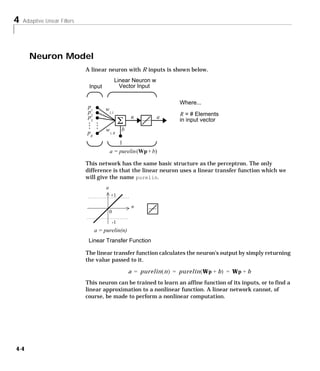
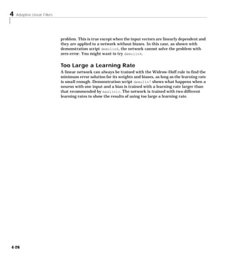
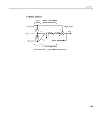
Prediction Example
Suppose that we would like to use an adaptive filter to predict the next value
of a stationary random process, p(t). We will use the network shown below to
do this.
Input Linear Digital Filter
p1(t) = p(t) Target = p(t)
D +
w1,2 e(t)
p2(t) = p(t - 1) n(t) a(t)
b -
D w1,3 1
p3(t) = p(t - 2) Adjust weights
a = purelin (Wp + b)
Predictive Filter: a(t) is approximation to p(t)
The signal to be predicted, p(t), enters from the left into a tapped delay line.
The previous two values of p(t) are available as outputs from the tapped delay
4-20](https://image.slidesharecdn.com/nnet-090922002848-phpapp01/85/Neural-Network-Toolbox-MATLAB-120-320.jpg)
![Adaptive Filtering (ADAPT)
line. The network uses adapt to change the weights on each time step so as to
minimize the error e(t) on the far right. If this error is zero, then the network
output a(t) is exactly equal to p(t), and the network has done its prediction
properly.
A detailed analysis of this network is not appropriate here, but we can state the
main points. Given the autocorrelation function of the stationary random
process p(t), the error surface, the maximum learning rate, and the optimum
values of the weights can be calculated. Commonly, of course, one does not have
detailed information about the random process, so these calculations cannot be
performed. But this lack does not matter to the network. The network, once
initialized and operating, adapts at each time step to minimize the error and
in a relatively short time is able to predict the input p(t).
Chapter 10 of [HDB96] presents this problem, goes through the analysis, and
shows the weight trajectory during training. The network finds the optimum
weights on its own without any difficulty whatsoever.
You also might want to try demonstration program nnd10nc to see an adaptive
noise cancellation program example in action. This demonstration allows you
to pick a learning rate and momentum, (see Chapter 5), and shows the learning
trajectory, and the original and cancellation signals verses time.
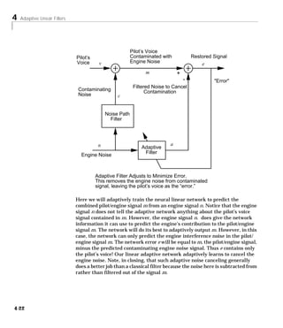
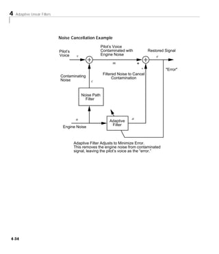
Noise Cancellation Example
Consider a pilot in an airplane. When the pilot speaks into as microphone, the
engine noise in the cockpit is added to the voice signal, and the resultant signal
heard by passengers would be of low quality. We would like to obtain a signal
which contains the pilot’s voice but not the engine noise. We can do this with
an adaptive filter if we can obtain a sample of the engine noise and apply it as
the input to the adaptive filter.
4-21](https://image.slidesharecdn.com/nnet-090922002848-phpapp01/85/Neural-Network-Toolbox-MATLAB-121-320.jpg)
![Limitations and Cautions
Limitations and Cautions
ADALINEs may only learn linear relationships between input and output
vectors. Thus ADALINEs cannot find solutions to some problems. However,
even if a perfect solution does not exist, the ADALINE will minimize the sum
of squared errors if the learning rate lr is sufficiently small. The network will
find as close a solution as is possible given the linear nature of the network’s
architecture. This property holds because the error surface of a linear network
is a multi-dimensional parabola. Since parabolas have only one minimum, a
gradient descent algorithm (such as the LMS rule) must produce a solution at
that minimum.
ADALINES have other various limitations. Some of them are discussed below.
Overdetermined Systems
Linear networks have a number of limitations. For instance, the system may
be overdetermined. Suppose that we have a network to be trained with four
1-element input vectors and four targets. A perfect solution to wp + b = t for
each of the inputs may not exist, for there are four constraining equations and
only one weight and one bias to adjust. However, the LMS rule will still
minimize the error. You might try demolin4 to see how this is done.
Underdetermined Systems
Consider a single linear neuron with one input. This time, in demolin5, we will
train it on only one 1-element input vector and its 1-element target vector:
P = [+1.0];
T = [+0.5];
Note that while there is only one constraint arising from the single input/target
pair, there are two variables, the weight and the bias. Having more variables
than constraints results in an underdetermined problem with an infinite
number of solutions. You might wish to try demoin5 to explore this topic.
Linearly Dependent Vectors
Normally it is a straightforward job to determine whether or not a linear
network can solve a problem. Commonly, if a linear network has at least as
many degrees of freedom (S*R+S = number of weights and biases) as
constraints (Q = pairs of input/target vectors), then the network can solve the
4-25](https://image.slidesharecdn.com/nnet-090922002848-phpapp01/85/Neural-Network-Toolbox-MATLAB-125-320.jpg)
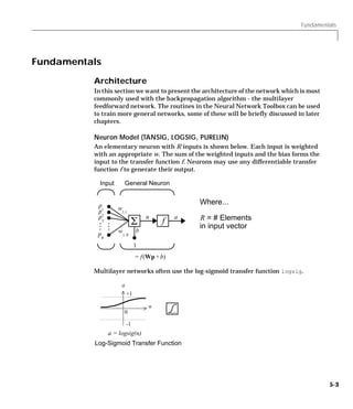
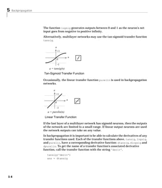
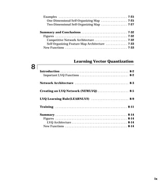
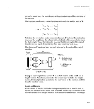
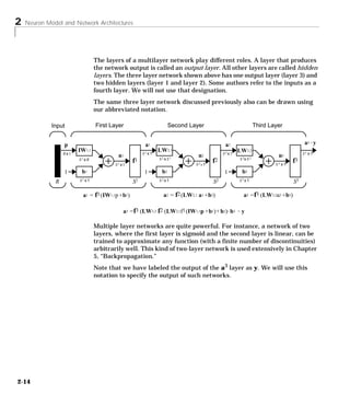
![5 Backpropagation
Input Hidden Layer Output Layer
p1 a1 a2
2 x1
IW1,1 4x1
LW2,1 3 x1
4x2
n1 3 x4
n2
4 x1 3 x1
f2
1 b1 1 b 2
2 4 x1 4 3 x1 3
a1 = tansig (IW1,1p1 +b1) a2 =purelin (LW2,1a1 +b2)
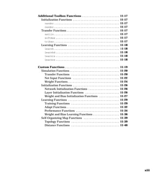
This network can be used as a general function approximator. It can
approximate any function with a finite number of discontinuities, arbitrarily
well, given sufficient neurons in the hidden layer.
Creating a Network (NEWFF). The first step in training a feedforward network is to
create the network object. The function newff creates a trainable feedforward
network. It requires four inputs and returns the network object. The first input
is an R by 2 matrix of minimum and maximum values for each of the R
elements of the input vector. The second input is an array containing the sizes
of each layer. The third input is a cell array containing the names of the
transfer functions to be used in each layer. The final input contains the name
of the training function to be used.
For example, the following command will create a two-layer network. There
will be one input vector with two elements, three neurons in the first layer and
one neuron in the second (output) layer. The transfer function in the first layer
will be tan-sigmoid, and the output layer transfer function will be linear. The
values for the first element of the input vector will range between -1 and 2, the
values of the second element of the input vector will range between 0 and 5, and
the training function will be traingd (which will be described in a later
section).
net=newff([-1 2; 0 5],[3,1],{'tansig','purelin'},'traingd');
This command creates the network object and also initializes the weights and
biases of the network; therefore the network is ready for training. There are
times when you may wish to re-initialize the weights, or to perform a custom
initialization. The next section explains the details of the initialization process.
5-6](https://image.slidesharecdn.com/nnet-090922002848-phpapp01/85/Neural-Network-Toolbox-MATLAB-142-320.jpg)
![Fundamentals
Initializing Weights (INIT, INITNW, RANDS). Before training a feedforward network,
the weights and biases must be initialized. The initial weights and biases are
created with the command init. This function takes a network object as input
and returns a network object with all weights and biases initialized. Here is
how a network is initialized:
net = init(net);
The specific technique which is used to initialize a given network will depend
on how the network parameters net.initFcn and net.layers{i}.initFcn are
set. The parameter net.initFcn is used to determine the overall initialization
function for the network. The default initialization function for the feedforward
network is initlay, which allows each layer to use its own initialization
function. With this setting for net.initFcn, the parameters
net.layers{i}.initFcn are used to determine the initialization method for
each layer.
For feedforward networks there are two different layer initialization methods
which are normally used: initwb and initnw. The initwb function causes the
initialization to revert to the individual initialization parameters for each
weight matrix (net.inputWeights{i,j}.initFcn) and bias. For the
feedforward networks the weight initialization is usually set to rands, which
sets weights to random values between -1 and 1. It is normally used when the
layer transfer function is linear.
The function initnw is normally used for layers of feedforward networks where
the transfer function is sigmoid. It is based on the technique of Nguyen and
Widrow [NgWi90] and generates initial weight and bias values for a layer so
that the active regions of the layer's neurons will be distributed roughly evenly
over the input space. It has several advantages over purely random weights
and biases: (1) few neurons are wasted (since the active regions of all the
neurons are in the input space), (2) training works faster (since each area of the
input space has active neuron regions).
The initialization function init is called by newff, therefore the network is
automatically initialized with the default parameters when it is created, and
init does not have to be called separately. However, the user may want to
re-initialize the weights and biases, or to use a specific method of initialization.
For example, in the network that we just created, using newff, the default
initialization for the first layer would be initnw. If we wanted to re-initialize
5-7](https://image.slidesharecdn.com/nnet-090922002848-phpapp01/85/Neural-Network-Toolbox-MATLAB-143-320.jpg)
![5 Backpropagation
the weights and biases in the first layer using the rands function, we would
issue the following commands:
net.layers{1}.initFcn = 'initwb';
net.inputWeights{1,1}.initFcn = 'rands';
net.biases{1,1}.initFcn = 'rands';
net.biases{2,1}.initFcn = 'rands';
net = init(net);
Simulation (SIM)
The function sim simulates a network. sim takes the network input p, and the
network object net, and returns the network outputs a. Here is how simuff can
be used to simulate the network we created above for a single input vector:
p = [1;2];
a = sim(net,p)
a =
-0.1011
(If you try these commands, your output may be different, depending on the
state of your random number generator when the network was initialized.)
Below, sim is called to calculate the outputs for a concurrent set of three input
vectors.
p = [1 3 2;2 4 1];
a=sim(net,p)
a =
-0.1011 -0.2308 0.4955
Training
Once the network weights and biases have been initialized, the network is
ready for training. The network can be trained for function approximation
(nonlinear regression), pattern association, or pattern classification. The
training process requires a set of examples of proper network behavior -
network inputs p and target outputs t. During training the weights and biases
of the network are iteratively adjusted to minimize the network performance
function net.performFcn. The default performance function for feedforward
networks is mean square error mse - the average squared error between the
network outputs a and the target outputs t.
5-8](https://image.slidesharecdn.com/nnet-090922002848-phpapp01/85/Neural-Network-Toolbox-MATLAB-144-320.jpg)
![Fundamentals
The remainder of this chapter will describe several different training
algorithms for feedforward networks. All of these algorithms use the gradient
of the performance function to determine how to adjust the weights to
minimize performance. The gradient is determined using a technique called
backpropagation, which involves performing computations backwards through
the network. The backpropagation computation is derived using the chain rule
of calculus and is described in Chapter 11 of [HDB96]. The basic
backpropagation training algorithm, in which the weights are moved in the
direction of the negative gradient, is described in the next section. Later
sections will describe more complex algorithms that increase the speed of
convergence.
Backpropagation Algorithm
There are many variations of the backpropagation algorithm, several of which
will be discussed in this chapter. The simplest implementation of
backpropagation learning updates the network weights and biases in the
direction in which the performance function decreases most rapidly - the
negative of the gradient. One iteration of this algorithm can be written
xk + 1 = xk – α k gk ,
where x k is a vector of current weights and biases, g k is the current gradient,
and α k is the learning rate.
There are two different ways in which this gradient descent algorithm can be
implemented: incremental mode and batch mode. In the incremental mode, the
gradient is computed and the weights are updated after each input is applied
to the network. In the batch mode all of the inputs are applied to the network
before the weights are updated. The next section will describe the incremental
training, and the following section will describe batch training.
Incremental Training(ADAPT)
The function adapt is used to train networks in the incremental mode. This
function takes the network object and the inputs and the targets from the
training set, and returns the trained network object and the outputs and errors
of the network for the final weights and biases.
There are several network parameters which must be set in order guide the
incremental training. The first is net.adaptFcn, which determines which
incremental mode training function is to be used. The default for feedforward
5-9](https://image.slidesharecdn.com/nnet-090922002848-phpapp01/85/Neural-Network-Toolbox-MATLAB-145-320.jpg)
![5 Backpropagation
networks is adaptwb, which allows each weight and bias to assign its own
function. These individual learning functions for the weights and biases are set
by the parameters net.biases{i,j}.learnFcn,
net.inputWeights{i,j}.learnFcn, and net.layerWeights{i,j}.learnFcn.
Gradient Descent (LEARDGD). For the basic steepest (gradient) descent algorithm,
the weights and biases are moved in the direction of the negative gradient of
the performance function. For this algorithm, the individual learning function
parameters for the weights and biases are set to 'learngd'. The following
commands illustrate how these parameters are set for the feedforward network
we created earlier.
net.biases{1,1}.learnFcn = 'learngd';
net.biases{2,1}.learnFcn = 'learngd';
net.layerWeights{2,1}.learnFcn = 'learngd';
net.inputWeights{1,1}.learnFcn = 'learngd';
The function learngd has one learning parameter associated with it - the
learning rate lr. The changes to the weights and biases of the network are
obtained by multiplying the learning rate times the negative of the gradient.
The larger the learning rate, the bigger the step. If the learning rate is made
too large the algorithm will become unstable. If the learning rate is set too
small, the algorithm will take a long time to converge. See page 12-8 of
[HDB96] for a discussion of the choice of learning rate.
The learning rate parameter is set to the default value for each weight and bias
when the learnFcn is set to learngd, as in the code above, although you can
change its value if you desire. The following command demonstrates how you
can set the learning rate to 0.2 for the layer weights. The learning rate can be
set separately for each weight and bias.
net.layerWeights{2,1}.learnParam.lr= 0.2;
The final parameter to be set for sequential training is
net.adaptParam.passes, which determines the number of passes through the
training set during training. Here we set the number of passes to 200.
net.adaptParam.passes = 200;
5-10](https://image.slidesharecdn.com/nnet-090922002848-phpapp01/85/Neural-Network-Toolbox-MATLAB-146-320.jpg)
![Fundamentals
We are now almost ready to train the network. It remains to set up the training
set. Here is a simple set of inputs and targets which we will use to illustrate
the training procedure:
p = [-1 -1 2 2;0 5 0 5];
t = [-1 -1 1 1];
If we want the learning algorithm to update the weights after each input
pattern is presented, we need to convert the matrices of inputs and targets into
cell arrays, with a cell for each input vector and target:
p = num2cell(p,1);
t = num2cell(t,1);
We are now ready to perform the incremental training using the adapt
function:
[net,a,e]=adapt(net,p,t);
After the training is complete we can simulate the network to test the quality
of the training.
a = sim(net,p)
a =
[-0.9995] [-1.0000] [1.0001] [1.0000]
Gradient Descent With Momentum (LEARDGDM). In addition to learngd, there is
another incremental learning algorithm for feedforward networks that often
provides faster convergence - learngdm, steepest descent with momentum.
Momentum allows a network to respond not only to the local gradient, but also
to recent trends in the error surface. Acting like a low pass filter, momentum
allows the network to ignore small features in the error surface. Without
momentum a network may get stuck in a shallow local minimum. With
momentum a network can slide through such a minimum. See page 12-9 of
[HDB96] for a discussion of momentum.
Momentum can be added to backpropagation learning by making weight
changes equal to the sum of a fraction of the last weight change and the new
change suggested by the backpropagation rule. The magnitude of the effect
that the last weight change is allowed to have is mediated by a momentum
constant, mc, which can be any number between 0 and 1. When the momentum
constant is 0 a weight change is based solely on the gradient. When the
5-11](https://image.slidesharecdn.com/nnet-090922002848-phpapp01/85/Neural-Network-Toolbox-MATLAB-147-320.jpg)
![5 Backpropagation
momentum constant is 1 the new weight change is set to equal the last weight
change and the gradient is simply ignored.
The learngdm function is invoked using the same steps shown above for the
learngd function, except that both the mc and lr learning parameters can be
set. Different parameter values can be used for each weight and bias, since
each weight and bias has its own learning parameters.
The following commands will cause the previously created network to be
incrementally trained using learngdm with the default learning parameters.
net.biases{1,1}.learnFcn = 'learngdm';
net.biases{2,1}.learnFcn = 'learngdm';
net.layerWeights{2,1}.learnFcn = 'learngdm';
net.inputWeights{1,1}.learnFcn = 'learngdm';
[net,a,e]=adapt(net,p,t);
Batch Training (TRAIN). The alternative to incremental training is batch training,
which is invoked using the function train. In batch mode the weights and
biases of the network are updated only after the entire training set has been
applied to the network. The gradients calculated at each training example are
added together to determine the change in the weights and biases. For a
discussion of batch training with the backpropagation algorithm see page 12-7
of [HDB96].
Batch Gradient Descent (TRAINGD). The batching equivalent of the incremental
function learngd is traingd, which implements the batching form of the
standard steepest descent training function. The weights and biases are
updated in the direction of the negative gradient of the performance function.
If you wish to train a network using batch steepest descent, you should set the
network trainFcn to traingd and then call the function train. Unlike the
learning functions in the previous section, which were assigned separately to
each weight matrix and bias vector in the network, there is only one training
function associated with a given network.
There are seven training parameters associated with traingd: epochs, show,
goal, time, min_grad, max_fail, and lr. The learning rate lr has the same
meaning here as it did for learngd - it is multiplied times the negative of the
gradient to determine the changes to the weights and biases. The training
status will be displayed every show iterations of the algorithm. The other
parameters determine when the training is stopped. The training will stop if
the number of iterations exceeds epochs, if the performance function drops
5-12](https://image.slidesharecdn.com/nnet-090922002848-phpapp01/85/Neural-Network-Toolbox-MATLAB-148-320.jpg)
![Fundamentals
below goal, if the magnitude of the gradient is less than mingrad, or if the
training time is longer than time seconds. We will discuss max_fail, which is
associated with the early stopping technique, in the section on improving
generalization.
The following code will recreate our earlier network, and then train it using
batch steepest descent. (Note that for batch training all of the inputs in the
training set are placed in one matrix.)
net=newff([-1 2; 0 5],[3,1],{'tansig','purelin'},'traingd');
net.trainParam.show = 50;
net.trainParam.lr = 0.05;
net.trainParam.epochs = 300;
net.trainParam.goal = 1e-5;
p = [-1 -1 2 2;0 5 0 5];
t = [-1 -1 1 1];
net=train(net,p,t);
TRAINGD, Epoch 0/300, MSE 1.59423/1e-05, Gradient 2.76799/
1e-10
TRAINGD, Epoch 50/300, MSE 0.00236382/1e-05, Gradient
0.0495292/1e-10
TRAINGD, Epoch 100/300, MSE 0.000435947/1e-05, Gradient
0.0161202/1e-10
TRAINGD, Epoch 150/300, MSE 8.68462e-05/1e-05, Gradient
0.00769588/1e-10
TRAINGD, Epoch 200/300, MSE 1.45042e-05/1e-05, Gradient
0.00325667/1e-10
TRAINGD, Epoch 211/300, MSE 9.64816e-06/1e-05, Gradient
0.00266775/1e-10
TRAINGD, Performance goal met.
a = sim(net,p)
a =
-1.0010 -0.9989 1.0018 0.9985
Try the Neural Network Design Demonstration nnd12sd1[HDB96] for an
illustration of the performance of the batch gradient descent algorithm.
Batch Gradient Descent With Momentum (TRAINGDM). The batch form of gradient
descent with momentum is invoked using the training function traingdm. This
algorithm is equivalent to learngdm, with two exceptions. First, the gradient is
computed by summing the gradients calculated at each training example, and
5-13](https://image.slidesharecdn.com/nnet-090922002848-phpapp01/85/Neural-Network-Toolbox-MATLAB-149-320.jpg)
![5 Backpropagation
the weights and biases are only updated after all training examples have been
presented. Second, if the new performance function on a given iteration
exceeds the performance function on a previous iteration by more than a
predefined ratio max_perf_inc (typically 1.04), the new weights and biases are
discarded, and the momentum coefficient mc is set to zero.
In the following code we recreate our previous network and retrain it using
gradient descent with momentum. The training parameters for traingdm are
the same as those for traingd, with the addition of the momentum factor mc
and the maximum performance increase max_perf_inc. (The training
parameters are reset to the default values whenever net.trainFcn is set to
traingdm.)
net=newff([-1 2; 0 5],[3,1],{'tansig','purelin'},'traingdm');
net.trainParam.show = 50;
net.trainParam.lr = 0.05;
net.trainParam.mc = 0.9;
net.trainParam.epochs = 300;
net.trainParam.goal = 1e-5;
p = [-1 -1 2 2;0 5 0 5];
t = [-1 -1 1 1];
net=train(net,p,t);
TRAINGDM, Epoch 0/300, MSE 3.6913/1e-05, Gradient 4.54729/
1e-10
TRAINGDM, Epoch 50/300, MSE 0.00532188/1e-05, Gradient
0.213222/1e-10
TRAINGDM, Epoch 100/300, MSE 6.34868e-05/1e-05, Gradient
0.0409749/1e-10
TRAINGDM, Epoch 114/300, MSE 9.06235e-06/1e-05, Gradient
0.00908756/1e-10
TRAINGDM, Performance goal met.
a = sim(net,p)
a =
-1.0026 -1.0044 0.9969 0.9992
5-14](https://image.slidesharecdn.com/nnet-090922002848-phpapp01/85/Neural-Network-Toolbox-MATLAB-150-320.jpg)
![Fundamentals
Note that since we re-initialized the weights and biases before training, we
obtain a different mean square error than we did using traingd. If we were to
re-initialize and train again using traingdm, we would get yet a different mean
square error. The random choice of initial weights and biases will affect the
performance of the algorithm. If you wish to compare the performance of
different algorithms, you should test each using several different sets of initial
weights and biases.
Try the Neural Network Design Demonstration nnd12mo [HDB96] for an
illustration of the performance of the batch momentum algorithm.
5-15](https://image.slidesharecdn.com/nnet-090922002848-phpapp01/85/Neural-Network-Toolbox-MATLAB-151-320.jpg)
![5 Backpropagation
Faster Training
The previous section presented two backpropagation training algorithms:
gradient descent and gradient descent with momentum. These two methods
are often too slow for practical problems. In this section we will discuss several
high performance algorithms which can converge from ten to one hundred
times faster than the algorithms discussed previously. All of the algorithms in
this section operate in the batch mode and are invoked using train.
These faster algorithms fall into two main categories. The first category uses
heuristic techniques, which were developed from an analysis of the
performance of the standard steepest descent algorithm. One heuristic
modification is the momentum technique, which was presented in the previous
section. This section will discuss two more heuristic techniques: variable
learning rate backpropagation, traingda, and resilient backpropagation
trainrp.
The second category of fast algorithms uses standard numerical optimization
techniques. (See Chapter 9 of [HDB96] for a review of basic numerical
optimization.) Later in this section we will present three types of numerical
optimization techniques for neural network training: conjugate gradient
(traincgf, traincgp, traincgb, trainscg), quasi-Newton (trainbfg,
trainoss), and Levenberg-Marquardt (trainlm).
Variable Learning Rate (TRAINGDA, TRAINGDX)
With standard steepest descent, the learning rate is held constant throughout
training. The performance of the algorithm is very sensitive to the proper
setting of the learning rate. If the learning rate is set too high, the algorithm
may oscillate and become unstable. If the learning rate is too small, the
algorithm will take too long to converge. It is not practical to determine the
optimal setting for the learning rate before training, and, in fact, the optimal
learning rate changes during the training process, as the algorithm moves
across the performance surface.
The performance of the steepest descent algorithm can be improved if we allow
the learning rate to change during the training process. An adaptive learning
rate will attempt to keep the learning step size as large as possible while
keeping learning stable. The learning rate is made responsive to the
complexity of the local error surface.
5-16](https://image.slidesharecdn.com/nnet-090922002848-phpapp01/85/Neural-Network-Toolbox-MATLAB-152-320.jpg)
![Faster Training
An adaptive learning rate requires some changes in the training procedure
used by traingd. First, the initial network output and error are calculated. At
each epoch new weights and biases are calculated using the current learning
rate. New outputs and errors are then calculated.
As with momentum, if the new error exceeds the old error by more than a
predefined ratio max_perf_inc (typically 1.04), the new weights and biases are
discarded. In addition, the learning rate is decreased (typically by multiplying
by lr_dec = 0.7). Otherwise the new weights, etc., are kept. If the new error is
less than the old error, the learning rate is increased (typically by multiplying
by lr_inc = 1.05).
This procedure increases the learning rate, but only to the extent that the
network can learn without large error increases. Thus a near optimal learning
rate is obtained for the local terrain. When a larger learning rate could result
in stable learning, the learning rate is increased. When the learning rate is too
high to guarantee a decrease in error, it gets decreased until stable learning
resumes.
Try the Neural Network Design Demonstration nnd12vl [HDB96] for an
illustration of the performance of the variable learning rate algorithm.
5-17](https://image.slidesharecdn.com/nnet-090922002848-phpapp01/85/Neural-Network-Toolbox-MATLAB-153-320.jpg)
![5 Backpropagation
Backpropagation training with an adaptive learning rate is implemented with
the function traingda which is called just like traingd except for the
additional training parameters max_perf_inc, lr_dec, and lr_inc. Here is
how it is called to train our previous two-layer network:
net=newff([-1 2; 0 5],[3,1],{'tansig','purelin'},'traingda');
net.trainParam.show = 50;
net.trainParam.lr = 0.05;
net.trainParam.lr_inc = 1.05;
net.trainParam.epochs = 300;
net.trainParam.goal = 1e-5;
p = [-1 -1 2 2;0 5 0 5];
t = [-1 -1 1 1];
net=train(net,p,t);
TRAINGDA, Epoch 0/300, MSE 1.71149/1e-05, Gradient 2.6397/
1e-06
TRAINGDA, Epoch 44/300, MSE 7.47952e-06/1e-05, Gradient
0.00251265/1e-06
TRAINGDA, Performance goal met.
a = sim(net,p)
a =
-1.0036 -0.9960 1.0008 0.9991
The function traingdx combines adaptive learning rate with momentum
training. It is invoked in the same way as traingda, except that it has the
momentum coefficient mc as an additional training parameter.
Resilient Backpropagation (TRAINRP)
Multilayer networks typically use sigmoid transfer functions in the hidden
layers. These functions are often called squashing functions, since they
compress an infinite input range into a finite output range. Sigmoid functions
are characterized by the fact that their slope must approach zero as the input
gets large. This causes a problem when using steepest descent to train a
multilayer network with sigmoid functions, since the gradient can have a very
small magnitude, and therefore cause small changes in the weights and biases,
even though the weights and biases are far from their optimal values.
The purpose of the resilient backpropagation (Rprop) training algorithm is to
eliminate these harmful effects of the magnitudes of the partial derivatives.
Only the sign of the derivative is used to determine the direction of the weight
5-18](https://image.slidesharecdn.com/nnet-090922002848-phpapp01/85/Neural-Network-Toolbox-MATLAB-154-320.jpg)
![Faster Training
update; the magnitude of the derivative has no effect on the weight update. The
size of the weight change is determined by a separate update value. The update
value for each weight and bias is increased by a factor delt_inc whenever the
derivative of the performance function with respect to that weight has the
same sign for two successive iterations. The update value is decreased by a
factor delt_dec whenever the derivative with respect that weight changes sign
from the previous iteration. If the derivative is zero, then the update value
remains the same. Whenever the weights are oscillating the weight change will
be reduced. If the weight continues to change in the same direction for several
iterations, then the magnitude of the weight change will be increased. A
complete description of the Rprop algorithm is given in [ReBr93].
In the following code we recreate our previous network and train it using the
Rprop algorithm. The training parameters for trainrp are epochs, show, goal,
time, min_grad, max_fail, delt_inc, delt_dec, delta0, deltamax. We have
previously discussed the first eight parameters. The last two are the initial step
size and the maximum step size, respectively. The performance of Rprop is not
very sensitive to the settings of the training parameters. For the example below
we leave most of the training parameters at the default values. We do reduce
show below our previous value, because Rprop generally converges much faster
than the previous algorithms.
net=newff([-1 2; 0 5],[3,1],{'tansig','purelin'},'trainrp');
net.trainParam.show = 10;
net.trainParam.epochs = 300;
net.trainParam.goal = 1e-5;
p = [-1 -1 2 2;0 5 0 5];
t = [-1 -1 1 1];
net=train(net,p,t);
TRAINRP, Epoch 0/300, MSE 0.469151/1e-05, Gradient 1.4258/
1e-06
TRAINRP, Epoch 10/300, MSE 0.000789506/1e-05, Gradient
0.0554529/1e-06
TRAINRP, Epoch 20/300, MSE 7.13065e-06/1e-05, Gradient
0.00346986/1e-06
TRAINRP, Performance goal met.
a = sim(net,p)
a =
-1.0026 -0.9963 0.9978 1.0017
5-19](https://image.slidesharecdn.com/nnet-090922002848-phpapp01/85/Neural-Network-Toolbox-MATLAB-155-320.jpg)
![5 Backpropagation
Rprop is generally much faster than the standard steepest descent algorithm.
It also has the nice property that it requires only a modest increase in memory
requirements. We do need to store the update values for each weight and bias,
which is equivalent to storage of the gradient.
Conjugate Gradient Algorithms
The basic backpropagation algorithm adjusts the weights in the steepest
descent direction (negative of the gradient). This is the direction in which the
performance function is decreasing most rapidly. It turns out that, although
the function decreases most rapidly along the negative of the gradient, this
does not necessarily produce the fastest convergence. In the conjugate gradient
algorithms a search is performed along conjugate directions, which produces
generally faster convergence than steepest descent directions. In this section
we will present four different variations of conjugate gradient algorithms.
See page 12-14 of [HDB96] for a discussion of conjugate gradient algorithms
and their application to neural networks.
In most of the training algorithms that we have discussed up to this point, a
learning rate is used to determine the length of the weight update (step size).
In most of the conjugate gradient algorithms the step size is adjusted at each
iteration. A search is made along the conjugate gradient direction to determine
the step size which will minimize the performance function along that line.
There are five different search functions that are included in the toolbox, and
these will be discussed at the end of this section. Any of these search functions
can be used interchangeably with a variety of the training functions described
in the remainder of this chapter. Some search functions are best suited to
certain training functions, although the optimum choice can vary according to
the specific application. An appropriate default search function is assigned to
each training function, but this can be modified by the user.
Fletcher-Reeves Update (TRAINCGF)
All of the conjugate gradient algorithms start out by searching in the steepest
descent direction (negative of the gradient) on the first iteration.
p 0 = –g0
5-20](https://image.slidesharecdn.com/nnet-090922002848-phpapp01/85/Neural-Network-Toolbox-MATLAB-156-320.jpg)
![Faster Training
A line search is then performed to determine the optimal distance to move
along the current search direction:
xk + 1 = xk + αkpk
Then the next search direction is determined so that it is conjugate to previous
search directions. The general procedure for determining the new search
direction is to combine the new steepest descent direction with the previous
search direction:
p k = – gk + βk p k – 1
The various versions of conjugate gradient are distinguished by the manner in
which the constant β k is computed. For the Fletcher-Reeves update the
procedure is
T
gk g k
β k = -------------------------- .
-
T
gk – 1gk – 1
This is the ratio of the norm squared of the current gradient to the norm
squared of the previous gradient.
See [FlRe64] or [HDB96] for a discussion of the Fletcher-Reeves conjugate
gradient algorithm.
In the following code we re-initialize our previous network and retrain it using
the Fletcher-Reeves version of the conjugate gradient algorithm. The training
parameters for traincgf are epochs, show, goal, time, min_grad, max_fail,
srchFcn, scal_tol, alpha, beta, delta, gama, low_lim, up_lim, maxstep,
minstep, bmax. We have previously discussed the first six parameters. The
parameter srchFcn is the name of the line search function. It can be any of the
functions described later in this section (or a user-supplied function). The
remaining parameters are associated with specific line search routines and are
described later in this section. The default line search routine srchcha is used
in this example. traincgf generally converges in fewer iterations than
trainrp (although there is more computation required in each iteration).
5-21](https://image.slidesharecdn.com/nnet-090922002848-phpapp01/85/Neural-Network-Toolbox-MATLAB-157-320.jpg)
![5 Backpropagation
net=newff([-1 2; 0 5],[3,1],{'tansig','purelin'},'traincgf');
net.trainParam.show = 5;
net.trainParam.epochs = 300;
net.trainParam.goal = 1e-5;
p = [-1 -1 2 2;0 5 0 5];
t = [-1 -1 1 1];
net=train(net,p,t);
TRAINCGF-srchcha, Epoch 0/300, MSE 2.15911/1e-05, Gradient
3.17681/1e-06
TRAINCGF-srchcha, Epoch 5/300, MSE 0.111081/1e-05, Gradient
0.602109/1e-06
TRAINCGF-srchcha, Epoch 10/300, MSE 0.0095015/1e-05, Gradient
0.197436/1e-06
TRAINCGF-srchcha, Epoch 15/300, MSE 0.000508668/1e-05,
Gradient 0.0439273/1e-06
TRAINCGF-srchcha, Epoch 17/300, MSE 1.33611e-06/1e-05,
Gradient 0.00562836/1e-06
TRAINCGF, Performance goal met.
a = sim(net,p)
a =
-1.0001 -1.0023 0.9999 1.0002
The conjugate gradient algorithms are usually much faster than variable
learning rate backpropagation, and are sometimes faster than trainrp,
although the results will vary from one problem to another. The conjugate
gradient algorithms require only a little more storage than the simpler
algorithms, so they are often a good choice for networks with a large number of
weights.
Try the Neural Network Design Demonstration nnd12cg [HDB96] for an
illustration of the performance of a conjugate gradient algorithm.
Polak-Ribiére Update (TRAINCGP)
Another version of the conjugate gradient algorithm was proposed by Polak
and Ribiére. As with the Fletcher-Reeves algorithm, the search direction at
each iteration is determined by
pk = – g k + β k p k – 1 .
5-22](https://image.slidesharecdn.com/nnet-090922002848-phpapp01/85/Neural-Network-Toolbox-MATLAB-158-320.jpg)
![Faster Training
For the Polak-Ribiére update, the constant β k is computed by
T
∆g k – 1 g k
β k = -------------------------- .
-
T
gk – 1gk – 1
This is the inner product of the previous change in the gradient with the
current gradient divided by the norm squared of the previous gradient. See
[FlRe64] or [HDB96] for a discussion of the Polak-Ribiére conjugate gradient
algorithm.
In the following code we recreate our previous network and train it using the
Polak-Ribiére version of the conjugate gradient algorithm. The training
parameters for traincgp are the same as those for traincgf. The default line
search routine srchcha is used in this example. The parameters show and
epoch are set to the same values as they were for traincgf.
net=newff([-1 2; 0 5],[3,1],{'tansig','purelin'},'traincgp');
net.trainParam.show = 5;
net.trainParam.epochs = 300;
net.trainParam.goal = 1e-5;
p = [-1 -1 2 2;0 5 0 5];
t = [-1 -1 1 1];
net=train(net,p,t);
TRAINCGP-srchcha, Epoch 0/300, MSE 1.21966/1e-05, Gradient
1.77008/1e-06
TRAINCGP-srchcha, Epoch 5/300, MSE 0.227447/1e-05, Gradient
0.86507/1e-06
TRAINCGP-srchcha, Epoch 10/300, MSE 0.000237395/1e-05,
Gradient 0.0174276/1e-06
TRAINCGP-srchcha, Epoch 15/300, MSE 9.28243e-05/1e-05,
Gradient 0.00485746/1e-06
TRAINCGP-srchcha, Epoch 20/300, MSE 1.46146e-05/1e-05,
Gradient 0.000912838/1e-06
TRAINCGP-srchcha, Epoch 25/300, MSE 1.05893e-05/1e-05,
Gradient 0.00238173/1e-06
TRAINCGP-srchcha, Epoch 26/300, MSE 9.10561e-06/1e-05,
Gradient 0.00197441/1e-06
TRAINCGP, Performance goal met.
a = sim(net,p)
a =
-0.9967 -1.0018 0.9958 1.0022
5-23](https://image.slidesharecdn.com/nnet-090922002848-phpapp01/85/Neural-Network-Toolbox-MATLAB-159-320.jpg)
![5 Backpropagation
The traincgp routine has performance similar to traincgf. It is difficult to
predict which algorithm will perform best on a given problem. The storage
requirements for Polak-Ribiére (four vectors) are slightly larger than for
Fletcher-Reeves (three vectors).
Powell-Beale Restarts (TRAINCGB)
For all conjugate gradient algorithms, the search direction will be periodically
reset to the negative of the gradient. The standard reset point occurs when the
number of iterations is equal to the number of network parameters (weights
and biases), but there are other reset methods which can improve the efficiency
of training. One such reset method was proposed by Powell [Powe77], based on
an earlier version proposed by Beale [Beal72]. For this technique we will
restart if there is very little orthogonality left between the current gradient and
the previous gradient. This is tested with the following inequality:
T 2
g k – 1 g k ≥ 0.2 g k .
If this condition is satisfied, the search direction is reset to the negative of the
gradient.
In the following code we recreate our previous network and train it using the
Powell-Beale version of the conjugate gradient algorithm. The training
parameters for traincgb are the same as those for traincgf. The default line
search routine srchcha is used in this example. The parameters show and
epoch are set to the same values as they were for traincgf.
net=newff([-1 2; 0 5],[3,1],{'tansig','purelin'},'traincgb');
net.trainParam.show = 5;
net.trainParam.epochs = 300;
net.trainParam.goal = 1e-5;
p = [-1 -1 2 2;0 5 0 5];
t = [-1 -1 1 1];
net=train(net,p,t);
TRAINCGB-srchcha, Epoch 0/300, MSE 2.5245/1e-05, Gradient
3.66882/1e-06
TRAINCGB-srchcha, Epoch 5/300, MSE 4.86255e-07/1e-05, Gradient
0.00145878/1e-06
TRAINCGB, Performance goal met.
a = sim(net,p)
a =
-0.9997 -0.9998 1.0000 1.0014
5-24](https://image.slidesharecdn.com/nnet-090922002848-phpapp01/85/Neural-Network-Toolbox-MATLAB-160-320.jpg)
![Faster Training
The traincgb routine has performance which is somewhat better than
traincgp for some problems, although performance on any given problem is
difficult to predict. The storage requirements for the Powell-Beale algorithm
(six vectors) are slightly larger than for Polak-Ribiére (four vectors).
Scaled Conjugate Gradient (TRAINSCG)
Each of the conjugate gradient algorithms which we have discussed so far
require a line search at each iteration. This line search is computationally
expensive, since it requires that the network response to all training inputs be
computed several times for each search. The scaled conjugate gradient
algorithm (SCG), developed by Moller [Moll93], was designed to avoid the time
consuming line search.This algorithm is too complex to explain in a few lines,
but the basic idea is to combine the model-trust region approach, which is used
in the Levenberg-Marquardt algorithm described later, with the conjugate
gradient approach. See {Moll93] for a detailed explanation of the algorithm.
In the following code we re-initialize our previous network and retrain it using
the scaled conjugate gradient algorithm. The training parameters for trainscg
are epochs, show, goal, time, min_grad, max_fail, sigma, lambda. We have
previously discussed the first six parameters. The parameter sigma determines
the change in the weight for the second derivative approximation. The
parameter lambda regulates the indefiniteness of the Hessian. The parameters
show and epoch are set to 10 and 300, respectively.
net=newff([-1 2; 0 5],[3,1],{'tansig','purelin'},'trainscg');
net.trainParam.show = 10;
net.trainParam.epochs = 300;
net.trainParam.goal = 1e-5;
p = [-1 -1 2 2;0 5 0 5];
t = [-1 -1 1 1];
net=train(net,p,t);
TRAINSCG, Epoch 0/300, MSE 4.17697/1e-05, Gradient 5.32455/
1e-06
TRAINSCG, Epoch 10/300, MSE 2.09505e-05/1e-05, Gradient
0.00673703/1e-06
TRAINSCG, Epoch 11/300, MSE 9.38923e-06/1e-05, Gradient
0.0049926/1e-06
TRAINSCG, Performance goal met.
a = sim(net,p)
a =
-1.0057 -1.0008 1.0019 1.0005
5-25](https://image.slidesharecdn.com/nnet-090922002848-phpapp01/85/Neural-Network-Toolbox-MATLAB-161-320.jpg)
![5 Backpropagation
The trainscg routine may require more iterations to converge than the other
conjugate gradient algorithms, but the number of computations in each
iteration is significantly reduced because no line search is performed. The
storage requirements for the scaled conjugate gradient algorithm are about the
same as those of Fletcher-Reeves.
Line Search Routines
Several of the conjugate gradient and quasi-Newton algorithms require that a
line search be performed. In this section we describe five different line searches
which can be used. In order to use any of these search routines you simply set
the training parameter srchFcn equal to the name of the desired search
function, as has been described in previous sections. It is often difficult to
predict which of these routines will provide the best results for any given
problem, but we have set the default search function to an appropriate initial
choice for each training function, so you may never need to modify this
parameter.
Golden Section Search (SRCHGOL)
The golden section search srchgol is a linear search which does not require the
calculation of the slope. This routine begins by locating an interval in which the
minimum of the performance occurs. This is accomplished by evaluating the
performance at a sequence of points, starting at a distance of delta and
doubling in distance each step, along the search direction. When the
performance increases between two successive iterations, a minimum has been
bracketed. The next step is to reduce the size of the interval containing the
minimum. Two new points are located within the initial interval. The values of
the performance at these two points determines a section of the interval which
can be discarded, and a new interior point is placed within the new interval.
This procedure is continued until the interval of uncertainty is reduced to a
width of tol, which is equal to delta/scale_tol.
See [HDB96], starting on page 12-16, for a complete description of the golden
section search. Try the Neural Network Design Demonstration nnd12sd1
[HDB96] for an illustration of the performance of the golden section search in
combination with a conjugate gradient algorithm.
5-26](https://image.slidesharecdn.com/nnet-090922002848-phpapp01/85/Neural-Network-Toolbox-MATLAB-162-320.jpg)
![Faster Training
Brent’s Search (SRCHBRE)
Brent’s search is a linear search which is a hybrid combination of the golden
section search and a quadratic interpolation. Function comparison methods,
like the golden section search, have a first-order rate of convergence, while
polynomial interpolation methods have an asymptotic rate which is faster than
superlinear. On the other hand, the rate of convergence for the golden section
search starts when the algorithm is initialized, whereas the asymptotic
behavior for the polynomial interpolation methods may take many iterations
to become apparent. Brent’s search attempts to combine the best features of
both approaches.
For Brent’s search we begin with the same interval of uncertainty that we used
with the golden section search, but some additional points are computed. A
quadratic function is then fitted to these points and the minimum of the
quadratic function is computed. If this minimum is within the appropriate
interval of uncertainty, it is used in the next stage of the search and a new
quadratic approximation is performed. If the minimum falls outside the known
interval of uncertainty, then a step of the golden section search is performed.
See [Bren73] for a complete description of this algorithm. This algorithm has
the advantage that it does not require computation of the derivative. The
derivative computation requires a backpropagation through the network,
which involves more computation than a forward pass. However, the algorithm
may require more performance evaluations than algorithms which use
derivative information.
Hybrid Bisection-Cubic Search (SRCHHYB)
Like Brent’s search, srchhyb is a hybrid algorithm. It is a combination of
bisection and cubic interpolation. For the bisection algorithm, one point is
located in the interval of uncertainty and the performance and its derivative
are computed. Based on this information, half of the interval of uncertainty is
discarded. In the hybrid algorithm, a cubic interpolation of the function is
obtained by using the value of the performance and its derivative at the two
end points. If the minimum of the cubic interpolation falls within the known
interval of uncertainty, then it is used to reduce the interval of uncertainty.
Otherwise, a step of the bisection algorithm is used.
See [Scal85] for a complete description of the hybrid bisection-cubic search.
This algorithm does require derivative information, so it performs more
computations at each step of the algorithm than the golden section search or
Brent’s algorithm.
5-27](https://image.slidesharecdn.com/nnet-090922002848-phpapp01/85/Neural-Network-Toolbox-MATLAB-163-320.jpg)
![5 Backpropagation
Charalambous’ Search (SRCHCHA)
The method of Charalambous srchcha was designed to be used in combination
with a conjugate gradient algorithm for neural network training. Like the
previous two methods, it is a hybrid search. It uses a cubic interpolation,
together with a type of sectioning.
See [Char92] for a description of Charalambous’ search. We have used this
routine as the default search for most of the conjugate gradient algorithms,
since it appears to produce excellent results for many different problems. It
does require the computation of the derivatives (backpropagation) in addition
to the computation of performance, but it overcomes this limitation by locating
the minimum with fewer steps. This is not true for all problems, and you may
want to experiment with other line searches.
Backtracking (SRCHBAC)
The backtracking search routine srchbac is best suited to use with the
quasi-Newton optimization algorithms. It begins with a step multiplier of 1 and
then backtracks until an acceptable reduction in the performance is obtained.
On the first step it uses the value of performance at the current point and at a
step multiplier of 1, and also the derivative of performance at the current point,
to obtain a quadratic approximation to the performance function along the
search direction. The minimum of the quadratic approximation becomes a
tentative optimum point (under certain conditions) and the performance at this
point is tested. If the performance is not sufficiently reduced, a cubic
interpolation is obtained and the minimum of the cubic interpolation becomes
the new tentative optimum point. This process is continued until a sufficient
reduction in the performance is obtained.
The backtracking algorithm is described in [DeSc83]. It was used as the default
line search for the quasi-Newton algorithms, although it may not be the best
technique for all problems.
5-28](https://image.slidesharecdn.com/nnet-090922002848-phpapp01/85/Neural-Network-Toolbox-MATLAB-164-320.jpg)
![5 Backpropagation
net=newff([-1 2; 0 5],[3,1],{'tansig','purelin'},'trainbfg');
net.trainParam.show = 5;
net.trainParam.epochs = 300;
net.trainParam.goal = 1e-5;
p = [-1 -1 2 2;0 5 0 5];
t = [-1 -1 1 1];
net=train(net,p,t);
TRAINBFG-srchbac, Epoch 0/300, MSE 0.492231/1e-05, Gradient
2.16307/1e-06
TRAINBFG-srchbac, Epoch 5/300, MSE 0.000744953/1e-05, Gradient
0.0196826/1e-06
TRAINBFG-srchbac, Epoch 8/300, MSE 7.69867e-06/1e-05, Gradient
0.00497404/1e-06
TRAINBFG, Performance goal met.
a = sim(net,p)
a =
-0.9995 -1.0004 1.0008 0.9945
The BFGS algorithm is described in [DeSc83]. This algorithm requires more
computation in each iteration and more storage than the conjugate gradient
methods, although it generally converges in fewer iterations. The approximate
2 2
Hessian must be stored, and its dimension is n × n , where n is equal to the
number of weights and biases in the network. For very large networks it may
be better to use Rprop or one of the conjugate gradient algorithms. For smaller
networks, however, trainbfg can be an efficient training function.
One Step Secant Algorithm (TRAINOSS)
Since the BFGS algorithm requires more storage and computation in each
iteration than the conjugate gradient algorithms, there is need for a secant
approximation with smaller storage and computation requirements. The one
step secant (OSS) method is an attempt to bridge the gap between the
conjugate gradient algorithms and the quasi-Newton (secant) algorithms. This
algorithm does not store the complete Hessian matrix; it assumes that at each
iteration the previous Hessian was the identity matrix. This has the additional
advantage that the new search direction can be calculated without computing
a matrix inverse.
In the following code we re-initialize our previous network and retrain it using
the one step secant algorithm. The training parameters for trainoss are the
same as those for traincgf. The default line search routine srchbac is used in
5-30](https://image.slidesharecdn.com/nnet-090922002848-phpapp01/85/Neural-Network-Toolbox-MATLAB-166-320.jpg)
![Faster Training
this example. The parameters show and epoch are set to 10 and 300,
respectively.
net=newff([-1 2; 0 5],[3,1],{'tansig','purelin'},'trainoss');
net.trainParam.show = 5;
net.trainParam.epochs = 300;
net.trainParam.goal = 1e-5;
p = [-1 -1 2 2;0 5 0 5];
t = [-1 -1 1 1];
net=train(net,p,t);
TRAINOSS-srchbac, Epoch 0/300, MSE 0.665136/1e-05, Gradient
1.61966/1e-06
TRAINOSS-srchbac, Epoch 5/300, MSE 0.000321921/1e-05, Gradient
0.0261425/1e-06
TRAINOSS-srchbac, Epoch 7/300, MSE 7.85697e-06/1e-05, Gradient
0.00527342/1e-06
TRAINOSS, Performance goal met.
a = sim(net,p)
a =
-1.0035 -0.9958 1.0014 0.9997
The one step secant method is described in [Batt92]. This algorithm requires
less storage and computation per epoch than the BFGS algorithm. It requires
slightly more storage and computation per epoch than the conjugate gradient
algorithms. It can be considered a compromise between full quasi-Newton
algorithms and conjugate gradient algorithms.
Levenberg-Marquardt (TRAINLM)
Like the quasi-Newton methods, the Levenberg-Marquardt algorithm was
designed to approach second-order training speed without having to compute
the Hessian matrix. When the performance function has the form of a sum of
squares (as is typical in training feedforward networks), then the Hessian
matrix can be approximated as
T
H = J J,
and the gradient can be computed as
T
g = J e
5-31](https://image.slidesharecdn.com/nnet-090922002848-phpapp01/85/Neural-Network-Toolbox-MATLAB-167-320.jpg)
![5 Backpropagation
where J is the Jacobian matrix, which contains first derivatives of the network
errors with respect to the weights and biases, and e is a vector of network
errors. The Jacobian matrix can be computed through a standard
backpropagation technique (see [HaMe94]) that is much less complex than
computing the Hessian matrix.
The Levenberg-Marquardt algorithm uses this approximation to the Hessian
matrix in the following Newton-like update:
T –1 T
x k + 1 = x k – [ J J + µI ] J e.
When the scalar µ is zero, this is just Newton’s method, using the approximate
Hessian matrix. When µ is large, this becomes gradient descent with a small
step size. Newton’s method is faster and more accurate near an error
minimum, so the aim is to shift towards Newton’s method as quickly as
possible. Thus, µ is decreased after each successful step (reduction in
performance function) and is increased only when a tentative step would
increase the performance function. In this way, the performance function will
always be reduced at each iteration of the algorithm.
In the following code we re-initialize our previous network and retrain it using
the Levenberg-Marquardt algorithm. The training parameters for trainlm are
epochs, show, goal, time, min_grad, max_fail, mu, mu_dec, mu_inc, mu_max,
mem_reduc. We have discussed the first six parameters earlier. The parameter
mu is the initial value for µ. This value is multiplied by mu_dec whenever the
performance function is reduced by a step. It is multiplied by mu_inc whenever
a step would increase the performance function. If mu becomes larger than
mu_max, the algorithm is stopped. The parameter mem_reduc is used to control
5-32](https://image.slidesharecdn.com/nnet-090922002848-phpapp01/85/Neural-Network-Toolbox-MATLAB-168-320.jpg)
![Faster Training
the amount of memory used by the algorithm. It will be discussed in the next
section. The parameters show and epoch are set to 5 and 300, respectively.
net=newff([-1 2; 0 5],[3,1],{'tansig','purelin'},'trainlm');
net.trainParam.show = 5;
net.trainParam.epochs = 300;
net.trainParam.goal = 1e-5;
p = [-1 -1 2 2;0 5 0 5];
t = [-1 -1 1 1];
net=train(net,p,t);
TRAINLM, Epoch 0/300, MSE 2.7808/1e-05, Gradient 7.77931/1e-10
TRAINLM, Epoch 4/300, MSE 3.67935e-08/1e-05, Gradient
0.000808272/1e-10
TRAINLM, Performance goal met.
a = sim(net,p)
a =
-1.0000 -1.0000 1.0000 0.9996
The original description of the Levenberg-Marquardt algorithm is given in
[Marq63]. The application of Levenberg-Marquardt to neural network training
is described in [HaMe94] and starting on page 12-19 of [HDB96]. This
algorithm appears to be the fastest method for training moderate-sized
feedforward neural networks (up to several hundred weights). It also has a
very efficient MATLAB implementation, since the solution of the matrix
equation is a built-in function, so its attributes become even more pronounced
in a MATLAB setting.
Try the Neural Network Design Demonstration nnd12m [HDB96] for an
illustration of the performance of the batch gradient descent algorithm.
Reduced Memory Levenberg-Marquardt (TRAINLM)
The main drawback of the Levenberg-Marquardt algorithm is that it requires
the storage of some matrices which can be quite large for certain problems. The
size of the Jacobian matrix is Q × n , where Q is the number of training sets and
n is the number of weights and biases in the network. It turns out that this
matrix does not have to be computed and stored as a whole. For example, if we
were to divide the Jacobian into two equal submatrices we could compute the
approximate Hessian matrix as follows:
5-33](https://image.slidesharecdn.com/nnet-090922002848-phpapp01/85/Neural-Network-Toolbox-MATLAB-169-320.jpg)
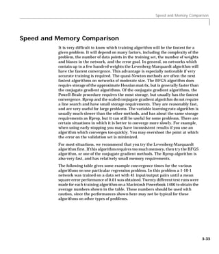
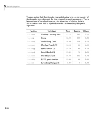
![Improving Generalization
Improving Generalization
One of the problems that occurs during neural network training is called
overfitting. The error on the training set is driven to a very small value, but
when new data is presented to the network the error is large. The network has
memorized the training examples, but it has not learned to generalize to new
situations.
The following figure shows the response of a 1-20-1 neural network which has
been trained to approximate a noisy sine function. The underlying sine
function is shown by the dotted line, the noisy measurements are given by the
‘+’ symbols, and the neural network response is given by the solid line. Clearly
this network has overfit the data and will not generalize well.
Function Approximation
1.5
1
0.5
Output
0
-0.5
-1
-1.5
-1 -0.8 -0.6 -0.4 -0.2 0 0.2 0.4 0.6 0.8 1
Input
One method for improving network generalization is to use a network which is
just large enough to provide an adequate fit. The larger a network you use, the
more complex the functions that the network can create. If we use a small
enough network, it will not have enough power to overfit the data. Run the
Neural Network Design Demonstration nnd11gn [HDB96] to investigate how
reducing the size of a network can prevent overfitting.
The problem is that it is difficult to know beforehand how large a network
should be for a specific application. There are two other methods for improving
5-37](https://image.slidesharecdn.com/nnet-090922002848-phpapp01/85/Neural-Network-Toolbox-MATLAB-173-320.jpg)
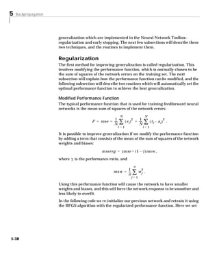
![Improving Generalization
the performance ratio to 0.5, which gives equal weight to the mean square
errors and the mean square weights.
net=newff([-1 2; 0 5],[3,1],{'tansig','purelin'},'trainbfg');
net.performFcn = 'msereg';
net.performParam.ratio = 0.5;
net.trainParam.show = 5;
net.trainParam.epochs = 300;
net.trainParam.goal = 1e-5;
p = [-1 -1 2 2;0 5 0 5];
t = [-1 -1 1 1];
net=train(net,p,t);
The problem with regularization is that it is difficult to determine the optimum
value for the performance ratio parameter. If we make this parameter too
large, we may get overfitting. If the ratio is too small, the network will not
adequately fit the training data. In the next section we will describe two
routines which automatically set the regularization parameters.
Automated Regularization (TRAINBR)
It is desirable to determine the optimal regularization parameters in an
automated fashion. One approach to this process is the Bayesian framework of
David MacKay [MacK92]. In this framework the weights and biases of the
network are assumed to be random variables with specified distributions. The
regularization parameters are related to the unknown variances associated
with these distributions. We can then estimate these parameters using
statistical techniques.
A detailed discussion of Bayesian regularization is beyond the scope of this
users guide. A detailed discussion of the use of Bayesian regularization, in
combination with Levenberg-Marquardt training, can be found in [FoHa97].
5-39](https://image.slidesharecdn.com/nnet-090922002848-phpapp01/85/Neural-Network-Toolbox-MATLAB-175-320.jpg)
![5 Backpropagation
Bayesian regularization has been implemented in the function trainbr. The
following code shows how we can train a 1-20-1 network using this function to
approximate the noisy sine wave shown earlier in this section.
net=newff([-1 1],[20,1],{'tansig','purelin'},'trainbr');
net.trainParam.show = 10;
net.trainParam.epochs = 50;
randn('seed',192736547);
p = [-1:.05:1];
t = sin(2*pi*p)+0.1*randn(size(p));
net = init(net);
net=train(net,p,t);
TRAINBR, Epoch 0/50, SSE 107.962/0, Gradient 9.51e+01/1.00e-10,
#Par 6.10e+01/61
TRAINBR, Epoch 10/50, SSE 20.5/0, Gradient 1.88e-01/1.00e-10,
#Par 1.82e+01/61
TRAINBR, Epoch 20/50, SSE 20.5/0, Gradient 4.07e-02/1.00e-10,
#Par 1.65e+01/61
TRAINBR, Epoch 30/50, SSE 20.5/0, Gradient 5.57e-01/1.00e-10,
#Par 1.55e+01/61
TRAINBR, Epoch 40/50, SSE 20.5/0, Gradient 2.76e-01/1.00e-10,
#Par 1.48e+01/61
TRAINBR, Epoch 50/50, SSE 20.5/0, Gradient 4.05e-01/1.00e-10,
#Par 1.42e+01/61
One feature of this algorithm is that it provides a measure of how many
network parameters (weights and biases) are being effectively used by the
network. In this case, the final trained network uses approximately 14
parameters (indicated by #Par in the printout), out of the 61 total weights and
biases in the 1-20-1 network. This effective number of parameters should
remain the same, no matter how large the total number of parameters in the
network becomes.
The following figure shows the response of the network. In contrast to the
previous figure, in which a 1-20-1 network overfit the data, here we see that
the network response is very close to the underlying sine function (dotted line),
and, therefore, the network will generalize well to new inputs. We could have
tried an even larger network, but the network response would never overfit the
data. This eliminates the guesswork required in determining the optimum
network size.
5-40](https://image.slidesharecdn.com/nnet-090922002848-phpapp01/85/Neural-Network-Toolbox-MATLAB-176-320.jpg)
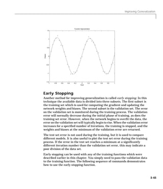
![5 Backpropagation
First we will create a simple test problem. For our training set we will generate
a noisy sine wave with input points ranging from -1 to 1 at steps of 0.05.
p = [-1:0.05:1];
t = sin(2*pi*p)+0.1*randn(size(p));
Next we will generate the validation set. The inputs will range from -1 to 1, as
in the test set, but we will offset them slightly. To make the problem more
realistic, we also add a different noise sequence to the underlying sine wave.
Notice that the validation set is contained in a structure which contains both
the inputs and the targets.
v.P = [-0.975:.05:0.975];
v.T = sin(2*pi*v.P)+0.1*randn(size(v.P));
We will now create a 1-20-1 network, as in our previous example with
regularization, and train it. (Notice that the validation structure is passed to
train after the initial input and layer conditions, which are null vectors in this
case since the network contains no delays.) For this example we will use the
training function traingdx, although early stopping can be used with any of
the other training functions we have discussed in this chapter.
net=newff([-1 1],[20,1],{'tansig','purelin'},'traingdx');
net.trainParam.show = 25;
net.trainParam.epochs = 300;
net = init(net);
[net,tr]=train(net,p,t,[],[],v);
TRAINGDX, Epoch 0/300, MSE 9.39342/0, Gradient 17.7789/1e-06
TRAINGDX, Epoch 25/300, MSE 0.312465/0, Gradient 0.873551/1e-06
TRAINGDX, Epoch 50/300, MSE 0.102526/0, Gradient 0.206456/1e-06
TRAINGDX, Epoch 75/300, MSE 0.0459503/0, Gradient 0.0954717/1e-06
TRAINGDX, Epoch 100/300, MSE 0.015725/0, Gradient 0.0299898/1e-06
TRAINGDX, Epoch 125/300, MSE 0.00628898/0, Gradient 0.042467/
1e-06
TRAINGDX, Epoch 131/300, MSE 0.00650734/0, Gradient 0.133314/
1e-06
TRAINGDX, Validation stop.
5-42](https://image.slidesharecdn.com/nnet-090922002848-phpapp01/85/Neural-Network-Toolbox-MATLAB-178-320.jpg)
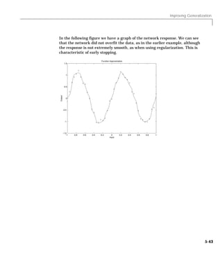
![5 Backpropagation
Preprocessing and Postprocessing
Neural network training can be made more efficient if certain preprocessing
steps are performed on the network inputs and targets. In this section we
describe several preprocessing routines which can be used.
Min and Max (PREMNMX, POSTMNMX, TRAMNMX)
Before training, it is often useful to scale the inputs and targets so that they
always fall within a specified range. The function premnmx can be used to scale
inputs and targets so that they fall in the range [-1,1]. The following code
illustrates the use of this function.
[pn,minp,maxp,tn,mint,maxt] = premnmx(p,t);
net=train(net,pn,tn);
The original network inputs and targets are given in the matrices p and t. The
normalized inputs and targets, pn and tn, that are returned will all fall in the
interval [-1,1]. The vectors minp and maxp contain the minimum and maximum
values of the original inputs, and the vectors mint and maxt contain the
minimum and maximum values of the original targets. After the network has
been trained, these vectors should be used to transform any future inputs
which are applied to the network. They effectively become a part of the
network, just like the network weights and biases.
If premnmx is used to scale both the inputs and targets, then the output of the
network will be trained to produce outputs in the range [-1,1]. If you want to
convert these outputs back into the same units which were used for the original
targets, then you should use the routine postmnmx. In the following code we
simulate the network which was trained in the previous code and then convert
the network output back into the original units.
an = sim(net,pn);
a = postmnmx(an,mint,maxt);
The network output an will correspond to the normalized targets tn. The
un-normalized network output a is in the same units as the original targets t.
If premnmx is used to preprocess the training set data, then whenever the
trained network is used with new inputs they should be preprocessed with the
minimum and maximums which were computed for the training set. This can
5-44](https://image.slidesharecdn.com/nnet-090922002848-phpapp01/85/Neural-Network-Toolbox-MATLAB-180-320.jpg)
![Preprocessing and Postprocessing
be accomplished with the routine tramnmx. In the following code we apply a new
set of inputs to the network we have already trained.
pnewn = tramnmx(pnew,minp,maxp);
anewn = sim(net,pnewn);
anew = postmnmx(anewn,mint,maxt);
Mean and Stand. Dev. (PRESTD, POSTSTD, TRASTD)
Another approach for scaling network inputs and targets is to normalize the
mean and standard deviation of the training set. This procedure is
implemented in the function prestd. It normalizes the inputs and targets so
that they will have zero mean and unity standard deviation. The following code
illustrates the use of prestd.
[pn,meanp,stdp,tn,meant,stdt] = prestd(p,t);
The original network inputs and targets are given in the matrices p and t. The
normalized inputs and targets, pn and tn, that are returned will have zero
means and unity standard deviation. The vectors meanp and stdp contain the
mean and standard deviations of the original inputs, and the vectors meant and
stdt contain the means and standard deviations of the original targets. After
the network has been trained, these vectors should be used to transform any
future inputs which are applied to the network. They effectively become a part
of the network, just like the network weights and biases.
If prestd is used to scale both the inputs and targets, then the output of the
network will be trained to produce outputs with zero mean and unity standard
deviation. If you want to convert these outputs back into the same units which
were used for the original targets, then you should use the routine poststd. In
the following code we simulate the network which was trained in the previous
code and then convert the network output back into the original units.
an = sim(net,pn);
a = poststd(an,meant,stdt);
The network output an will correspond to the normalized targets tn. The
un-normalized network output a is in the same units as the original targets t.
If prestd is used to preprocess the training set data, then whenever the trained
network is used with new inputs they should be preprocessed with the means
and standard deviations which were computed for the training set. This can be
5-45](https://image.slidesharecdn.com/nnet-090922002848-phpapp01/85/Neural-Network-Toolbox-MATLAB-181-320.jpg)
![5 Backpropagation
accomplished with the routine trastd. In the following code we apply a new set
of inputs to the network we have already trained.
pnewn = trastd(pnew,meanp,stdp);
anewn = sim(net,pnewn);
anew = poststd(anewn,meant,stdt);
Principal Component Analysis (PREPCA, TRAPCA)
In some situations the dimension of the input vector is large, but the
components of the vectors are highly correlated (redundant). It is useful in this
situation to reduce the dimension of the input vectors. An effective procedure
for performing this operation is principal component analysis. This technique
has three effects: it orthogonalizes the components of the input vectors (so that
they are uncorrelated with each other); it orders the resulting orthogonal
components (principal components) so that those with the largest variation
come first; and it eliminates those components which contribute the least to the
variation in the data set. The following code illustrates the use of prepca,
which performs a principal component analysis.
[pn,meanp,stdp] = prestd(p);
[ptrans,transMat] = prepca(pn,0.02);
Note that we first normalize the input vectors, using prestd, so that they have
zero mean and unity variance. This is a standard procedure when using
principal components. In this example, the second argument passed to prepca
is 0.02. This means that prepca will eliminate those principal components
which contribute less than 2% to the total variation in the data set. The matrix
ptrans contains the transformed input vectors. The matrix transMat contains
the principal component transformation matrix. After the network has been
trained, this matrix should be used to transform any future inputs which are
applied to the network. It effectively becomes a part of the network, just like
the network weights and biases. If you multiply the normalized input vectors
pn by the transformation matrix transMat, you will obtain the transformed
input vectors ptrans.
If prepca is used to preprocess the training set data, then whenever the trained
network is used with new inputs they should be preprocessed with the
transformation matrix which was computed for the training set.
5-46](https://image.slidesharecdn.com/nnet-090922002848-phpapp01/85/Neural-Network-Toolbox-MATLAB-182-320.jpg)
![Preprocessing and Postprocessing
This can be accomplished with the routine trapca. In the following code we
apply a new set of inputs to a network we have already trained.
pnewn = trastd(pnew,meanp,stdp);
pnewtrans = trapca(pnewn,transMat);
a = sim(net,pnewtrans);
Post-training Analysis (POSTREG)
The performance of a trained network can be measured to some extent by the
errors on the training, validation and test sets, but it is often useful to
investigate the network response in more detail. One option is to perform a
regression analysis between the network response and the corresponding
targets. The routine postreg is designed to perform this analysis.
The following commands illustrate how we can perform a regression analysis
on the network which we previously trained in the early stopping section.
a = sim(net,p);
[m,b,r] = postreg(a,t)
m =
0.9874
b =
-0.0067
r =
0.9935
Here we pass the network output and the corresponding targets to postreg. It
returns three parameters. The first two, m and b, correspond to the slope and
the y-intercept of the best linear regression relating targets to network
outputs. If we had a perfect fit (outputs exactly equal to targets), the slope
would be 1, and the y-intercept would be 0. In this example we can see that the
numbers are very close. The third variable returned by postreg is the
correlation coefficient (R-value) between the outputs and targets. It is a
measure of how well the variation in the output is explained by the targets. If
this number is equal to 1, then there is perfect correlation between targets and
outputs. In our example here the number is very close to 1, which indicates a
good fit.
The following figure illustrates the graphical output provided by postreg. The
network outputs are plotted versus the targets as open circles. The best linear
fit is indicated by a dashed line. The perfect fit (output equal to targets) is
5-47](https://image.slidesharecdn.com/nnet-090922002848-phpapp01/85/Neural-Network-Toolbox-MATLAB-183-320.jpg)
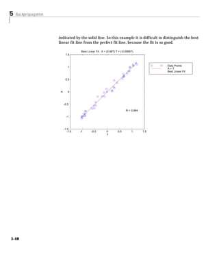
![Sample Training Session
Sample Training Session
We have covered a number of different concepts in this chapter. At this point it
might be useful to put some of these ideas together with an example of how a
typical training session might go.
For this example we are going to use data from a medical application [PuLu92].
We want to design an instrument which can determine serum cholesterol levels
from measurements of spectral content of a blood sample. We have a total of
264 patients for which we have measurements of 21 wavelengths of the
spectrum. For the same patients we also have measurements of hdl, ldl and
vldl cholesterol levels, based on serum separation. The first step is to load the
data into the workspace and perform a principal component analysis.
load choles_all
[pn,meanp,stdp,tn,meant,stdt] = prestd(p,t);
[ptrans,transMat] = prepca(pn,0.001);
Here we have conservatively retained those principal components which
account for 99.9% of the variation in the data set. Let’s check the size of the
transformed data.
[R,Q] = size(ptrans)
R =
4
Q =
264
There was apparently significant redundancy in the data set, since the
principal component analysis has reduced the size of the input vectors from 21
to 4.
The next step is to divide the data up into training, validation and test subsets.
We will take one fourth of the data for the validation set, one fourth for the test
set and one half for the training set. We will pick the sets as equally spaced
points throughout the original data.
iitst = 2:4:Q;
iival = 4:4:Q;
iitr = [1:4:Q 3:4:Q];
v.P = ptrans(:,iival); v.T = tn(:,iival);
t.P = ptrans(:,iitst); t.V = tn(:,iitst);
ptr = ptrans(:,iitr); ttr = tn(:,iitr);
5-49](https://image.slidesharecdn.com/nnet-090922002848-phpapp01/85/Neural-Network-Toolbox-MATLAB-185-320.jpg)
![5 Backpropagation
We are now ready to create a network and train it. For this example we will try
a two-layer network, with tan-sigmoid transfer function in the hidden layer
and a linear transfer function in the output layer. This is a useful structure for
function approximation (or regression) problems. As an initial guess, we will
use five neurons in the hidden layer. The network should have three output
neurons since there are three targets. We will use the Levenberg-Marquardt
algorithm for training.
net = newff(minmax(ptr),[5 3],{'tansig' 'purelin'},'trainlm');
[net,tr]=train(net,ptr,ttr,[],[],v,t);
TRAINLM, Epoch 0/100, MSE 3.11023/0, Gradient 804.959/1e-10
TRAINLM, Epoch 15/100, MSE 0.330295/0, Gradient 104.219/1e-10
TRAINLM, Validation stop.
The training stopped after 15 iterations because the validation error increased.
It is a useful diagnostic tool to plot the training, validation and test errors to
check the progress of training. We can do that with the following commands.
plot(tr.epoch,tr.perf,tr.epoch,tr.vperf,tr.epoch,tr.tperf)
legend('Training','Validation','Test',-1);
ylabel('Squared Error'); xlabel('Epoch')
The result is shown in the following figure. The result here is reasonable, since
the test set error and the validation set error have similar characteristics, and
it doesn’t appear that any significant overfitting has occurred.
5-50](https://image.slidesharecdn.com/nnet-090922002848-phpapp01/85/Neural-Network-Toolbox-MATLAB-186-320.jpg)
![Sample Training Session
3.5
3
Training
Validation
2.5 Test
Squared Error
2
1.5
1
0.5
0
0 5 10 15
Epoch
The next step is to perform some analysis of the network response. We will put
the entire data set through the network (training, validation and test) and will
perform a linear regression between the network outputs and the
corresponding targets. First we will need to un-normalize the network outputs.
an = sim(net,ptrans);
a = poststd(an,meant,stdt);
for i=1:3
figure(i)
[m(i),b(i),r(i)] = postreg(a(i,:),t(i,:));
end
In this case we have three outputs, so we perform three regressions. The
results are shown in the following figures.
5-51](https://image.slidesharecdn.com/nnet-090922002848-phpapp01/85/Neural-Network-Toolbox-MATLAB-187-320.jpg)
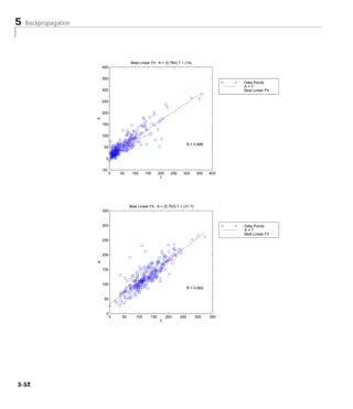
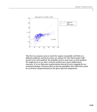
![5 Backpropagation
Limitations and Cautions
The gradient descent algorithm is generally very slow, because it requires
small learning rates for stable learning. The momentum variation is usually
faster than simple gradient descent, since it allows higher learning rates while
maintaining stability, but it is still too slow for many practical applications.
These two methods would normally be used only when incremental training is
desired. You would normally use Levenberg-Marquardt training if you have
enough memory available. If memory is a problem, then there are a variety of
other fast algorithms available.
Multi-layered networks are capable of performing just about any linear or
nonlinear computation, and can approximate any reasonable function
arbitrarily well. Such networks overcome the problems associated with the
perceptron and linear networks. However, while the network being trained
may be capable theoretically of performing correctly, backpropagation and its
variations may not always find a solution. See page 12-8 of [HDB96] for a
discussion of convergence to local minimum points.
Picking the learning rate for a nonlinear network is a challenge. As with linear
networks, a learning rate that is too large leads to unstable learning.
Conversely, a learning rate that is too small results in incredibly long training
times. Unlike linear networks, there is no easy way of picking a good learning
rate for nonlinear multilayer networks. See page 12-8 of [HDB96] for examples
of choosing the learning rate. With the faster training algorithms, the default
parameter values will normally perform adequately.
The error surface of a nonlinear network is more complex than the error
surface of a linear network. To understand this complexity see the figures on
pages 12-5 to 12-7 of [HDB96], which show three different error surfaces for a
multilayer network. The problem is that nonlinear transfer functions in
multilayer networks introduce many local minima in the error surface. As
gradient descent is performed on the error surface it is possible for the network
solution to become trapped in one of these local minima. This may happen
depending on the initial starting conditions. Settling in a local minimum may
be good or bad depending on how close the local minimum is to the global
minimum and how low an error is required. In any case, be cautioned that
although a multilayer backpropagation network with enough neurons can
implement just about any function, backpropagation will not always find the
correct weights for the optimum solution. You may wish to re-initialize the
network and retrain several times to guarantee that you have the best solution.
5-54](https://image.slidesharecdn.com/nnet-090922002848-phpapp01/85/Neural-Network-Toolbox-MATLAB-190-320.jpg)
![Limitations and Cautions
Networks are also sensitive to the number of neurons in their hidden layers.
Too few neurons can lead to underfitting. Too many neurons can contribute to
overfitting, in which all training points are well fit, but the fitting curve takes
wild oscillations between these points. Ways of dealing with various of these
issues have been discussed in the section on improving generalization. This
topic is also discussed starting on page 11-21 of [HDB96].
5-55](https://image.slidesharecdn.com/nnet-090922002848-phpapp01/85/Neural-Network-Toolbox-MATLAB-191-320.jpg)
![5 Backpropagation
In order to produce the most efficient training, it is often helpful to preprocess
the data before training. It is also helpful to analyze the network response after
training is complete. The toolbox contains a number of routines for pre- and
post-processing. They are summarized in the following table.
Function Description
premnmx Normalize data to fall in the range [-1,1].
postmnmx Inverse of premnmx. Used to convert data back to standard
units.
tramnmx Normalize data using previously computed minimums and
maximums. Used to preprocess new inputs to networks
which have been trained with data normalized with premnmx.
prestd Normalize data to have zero mean and unity standard
deviation.
poststd Inverse of prestd. Used to convert data back to standard
units.
trastd Normalize data using previously computed means and
standard deviations. Used to preprocess new inputs to
networks which have been trained with data normalized
with prestd.
prepca Principal component analysis. Reduces dimension of input
vector and un-correlates components of input vectors.
trapca Preprocess data using previously computed principal
component transformation matrix. Used to preprocess new
inputs to networks which have been trained with data
transformed with prepca.
postreg Linear regression between network outputs and targets.
Used to determine the adequacy of network fit.
5-58](https://image.slidesharecdn.com/nnet-090922002848-phpapp01/85/Neural-Network-Toolbox-MATLAB-194-320.jpg)
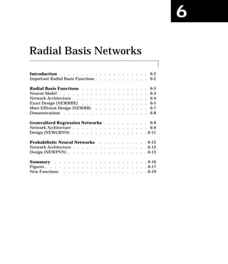
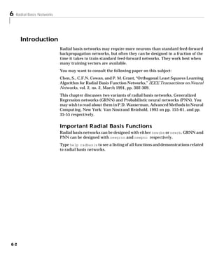
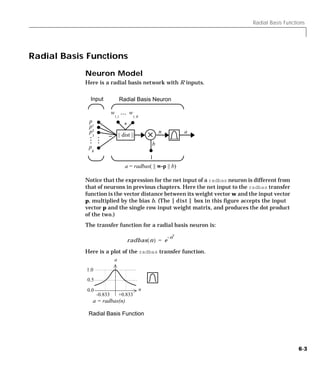
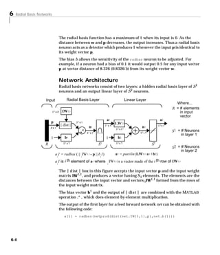

![6 Radial Basis Networks
This function newrbe creates as many radbas neurons as there are input
vectors in P, and sets the first layer weights to P'. Thus, we have a layer of
radbas neurons in which each neuron acts as a detector for a different input
vector. If there are Q input vectors, then there will be Q neurons.
Each bias in the first layer is set to 0.8326/SPREAD. This gives radial basis
functions that cross 0.5 at weighted inputs of +/- SPREAD. This determines the
width of an area in the input space to which each neuron responds. If SPREAD
is 4, then each radbas neuron will respond with 0.5 or more to any input vectors
within a vector distance of 4 from their weight vector. As we shall see, SPREAD
should be large enough that neurons respond strongly to overlapping regions
of the input space.
The second layer weights IW 2,1 (or in code, IW{2,1}) and biases b 2 (or in code,
b{2}) are found by simulating the first layer outputs a1 (A{1}), and then solving
the following linear expression:
[W{2,1} b{2}] * [A{1}; ones] = T
We know the inputs to the second layer (A{1}) and the target (T), and the layer
is linear. We can use the following code to calculate the weights and biases of
the second layer to minimize the sum-squared error.
Wb = T/[P; ones(1,Q)]
Here Wb contains both weights and biases, with the biases in the last column.
The sum-squared error will always be 0, as explained below.
We have a problem with C constraints (input/target pairs) and each neuron has
C +1 variables (the C weights from the C radbas neurons, and a bias). A linear
problem with C constraints and more than C variables has an infinite number
of zero error solutions!
Thus newrbe creates a network with zero error on training vectors. The only
condition we have to meet is to make sure that SPREAD is large enough so that
the active input regions of the radbas neurons overlap enough so that several
radbas neurons always have fairly large outputs at any given moment. This
makes the network function smoother and results in better generalization for
new input vectors occurring between input vectors used in the design.
(However, SPREAD should not be so large that each neuron is effectively
responding in the same, large, area of the input space.)
6-6](https://image.slidesharecdn.com/nnet-090922002848-phpapp01/85/Neural-Network-Toolbox-MATLAB-200-320.jpg)
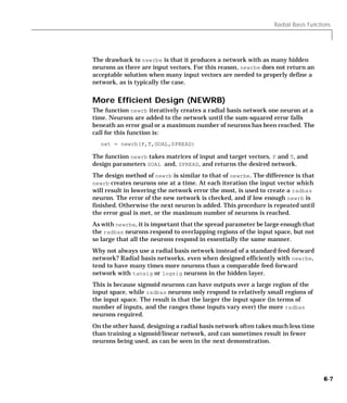

![Generalized Regression Networks
Generalized Regression Networks
A generalized regression neural network (GRNN) is often used for function
approximation. As discussed below, it has a radial basis layer and a special
linear layer.
Network Architecture
The architecture for the GRNN is shown below. It is similar to the radial basis
network, but has a slightly different second layer.
Input Radial Basis Layer Special Linear Layer Where...
R = # elements
Q xR IW1,1 in input vector
Q xQ LW2,1
a2 Q = # Neurons
p Q x1
|| dist || Q x1
in layer 1
Rx1 n 1 a1 n 2
.* Q x1 Q x1
nprod
Q x1 Q = # Neurons
1 b1 in layer 2
R Q x1 Q Q Q = # of input/
target pairs
a 1 = radbas ( || IW1,1 - p || b 1) a2 = purelin ( n2)
i i i
ai1 is i th element of a1 where i IW1,1 is a vector made of the i th row of IW1,1
Here the nprod box shown above (code function normprod) produces S2
elements in vector n2. Each element is the dot product of a row of LW2,1 and
the input vector a1, all normalized by the sum of the elements of a1. For
instance, suppose that:
LW{1,2}= [1 -2;3 4;5 6];
a{1} = [7; -8;
Then
aout = normprod(LW{1,2},a{1})
aout =
-23
11
13
6-9](https://image.slidesharecdn.com/nnet-090922002848-phpapp01/85/Neural-Network-Toolbox-MATLAB-203-320.jpg)

![Generalized Regression Networks
Design (NEWGRNN)
You can use the function newgrnn to create a GRNN. For instance, suppose that
three input and three target vectors are defined as:
P = [4 5 6];
T = [1.5 3.6 6.7];
We can now obtain a GRNN with:
net = newgrnn(P,T);
and simulate it with:
P = 4.5;
v = sim(net,P)
You might want to try demogrn1. It shows how to approximate a function with
a GRNN.
6-11](https://image.slidesharecdn.com/nnet-090922002848-phpapp01/85/Neural-Network-Toolbox-MATLAB-205-320.jpg)
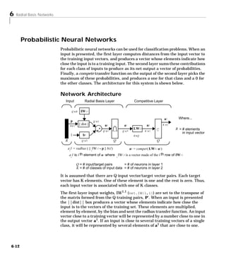
![Probabilistic Neural Networks
The second layer weights, LW1,2 (net.LW{2,1}), are set to the matrix T of
target vectors. Each vector has a one only in the row associated with that
particular class of input, and zeros elsewhere. (A function ind2vec is used to
create the proper vectors.) The multiplication Ta1 sums the elements of a1 due
to each of the K input classes. Finally, the second layer transfer function,
compete, produces a one corresponding to the largest element of n2, and zeros
elsewhere. Thus, the network has classified the input vector into a specific one
of K classes because that class had the maximum probability of being correct.
Design (NEWPNN)
You can use the function newpnn to create a PNN. For instance, suppose that
seven input vectors and their corresponding targets are:
P = [0 0;1 1;0 3;1 4;3 1;4 1;4 3]'
which yields
P =
0 1 0 1 3 4 4
0 1 3 4 1 1 3
Tc = [1 1 2 2 3 3 3];
Which yields
Tc =
1 1 2 2 3 3 3
We need a target matrix with ones in the right place. We can get it with the
function ind2vec. It gives a matrix with zeros except at the correct spots. So
execute
T = ind2vec(Tc)
which gives
T =
(1,1) 1
(1,2) 1
(2,3) 1
(2,4) 1
(3,5) 1
(3,6) 1
(3,7) 1
6-13](https://image.slidesharecdn.com/nnet-090922002848-phpapp01/85/Neural-Network-Toolbox-MATLAB-207-320.jpg)
![6 Radial Basis Networks
Now we can create a network and simulate it, using the input P to make sure
that it does produce the correct classifications. We will use the function
vec2ind to convert the output Y into a row Yc to make the classifications clear.
net = newpnn(P,T);
Y = sim(net,P)
Yc = vec2ind(Y)
Finally we get
Yc =
1 1 2 2 3 3 3
We might try classifying vectors other than those that were used to design the
network. We will try to classify the vectors shown below in P2.
P2 = [1 4;0 1;5 2]'
P2 =
1 0 5
4 1 2
Can you guess how these vectors will be classified? If we run the simulation
and plot the vectors as we did before we get:
Yc =
2 1 3
These results look good, for these test vectors were quite close to members of
classes 2, 1 and 3 respectively. The network has managed generalize its
operation to properly classify vectors other than those used to design the
network.
You might want to try demopnn1. It shows how to design a PNN, and how the
network can successfully classify a vector not used in the design.
6-14](https://image.slidesharecdn.com/nnet-090922002848-phpapp01/85/Neural-Network-Toolbox-MATLAB-208-320.jpg)
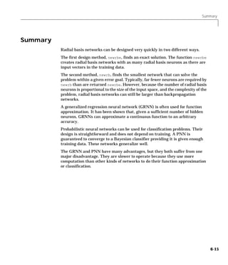
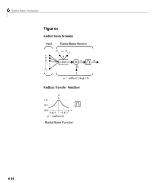
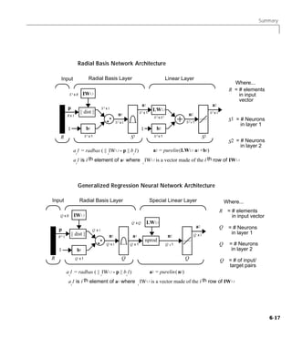
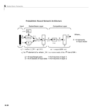

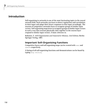
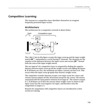
![7 Self-Organizing Networks
Creating a Competitive Neural Network (NEWC)
A competitive neural network can be created with the function newc. We will
show how this works with a simple example.
Suppose that we wish to divide the following four two element vectors into two
classes.
p = [.1 .8 .1 .9; .2 .9 .1 .8]
p =
0.1000 0.8000 0.1000 0.9000
0.2000 0.9000 0.1000 0.8000
Thus, we have two vectors near the origin and two vectors near (1,1).
First create a two neuron layer is created with two input elements ranging
from 0 to 1. The first argument gives the range of the two input vectors and the
second argument says that there are to be 2 neurons.
net = newc([0 1; 0 1],2);
The weights will be initialized to the center of the input ranges with the
function midpoint. We can check to see these initial values as follows:
wts = net.IW{1,1}
wts =
0.5000 0.5000
0.5000 0.5000
These weights are indeed the values at the midpoint of the range (0 to 1) of the
inputs, as we would expect when using midpoint for initialization.
The biases are computed by initcon, which gives
biases =
5.4366
5.4366
Now we have a network, but we need to train it to do the classification job.
Recall that each neuron competes to respond to an input vector p. If the biases
are all 0, the neuron whose weight vector is closest to p gets the highest net
input and therefore wins the competition and outputs 1. All other neurons
output 0. We would like to adjust the winning neuron so as to move it closer to
the input. A learning rule to do this is discussed in the next section.
7-4](https://image.slidesharecdn.com/nnet-090922002848-phpapp01/85/Neural-Network-Toolbox-MATLAB-218-320.jpg)
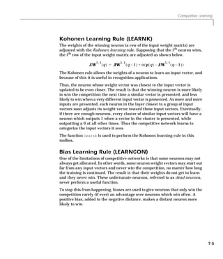
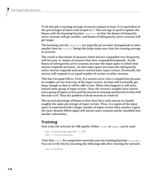
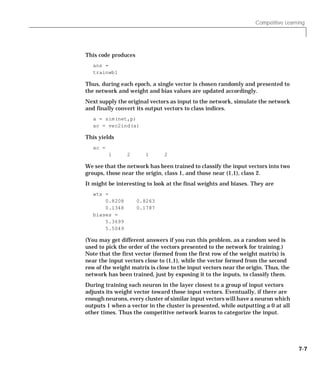
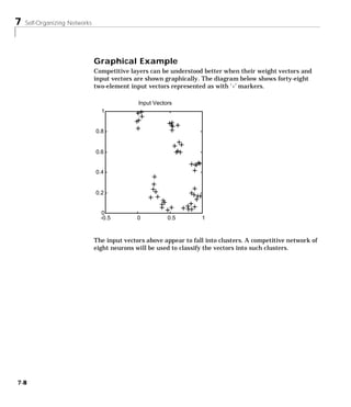
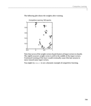

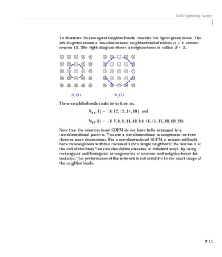
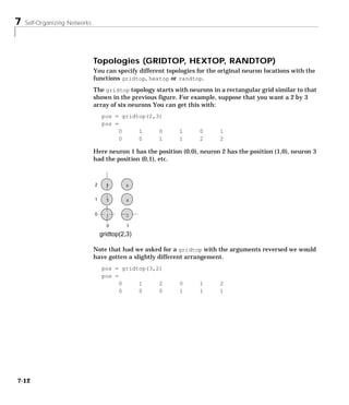
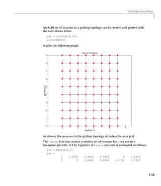
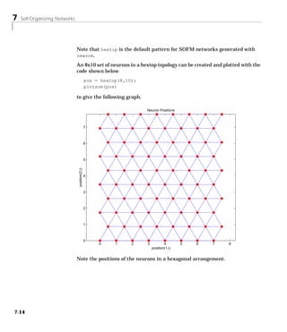
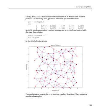
![7 Self-Organizing Networks
Distance Functions (DIST, LINKDIST, MANDIST,
BOXDIST)
In this toolbox there are four distinct ways to calculate distances from a
particular neuron to its neighbors. Each calculation method is implemented
with a special function.
The dist function has been discussed before. It calculates the Euclidean
distance from a home neuron to any other neuron. Suppose we have three
neurons:
pos2 = [ 0 1 2; 0 1 2]
pos2 =
0 1 2
0 1 2
We will find the distance from each neuron to the other with:
D2 = dist(pos2)
D2 =
0 1.4142 2.8284
1.4142 0 1.4142
2.8284 1.4142 0
Thus, the distance from neuron 1 to itself is 0, the distance from neuron 1 to
neuron 2 is 1.414, etc. These are indeed the Euclidean distances as we know
them.
The graph below shows a home neuron in a two-dimensional (gridtop) layer of
neurons. The home neuron has neighborhoods of increasing diameter
surrounding it. A neighborhood of diameter 1 includes the home neuron and its
7-16](https://image.slidesharecdn.com/nnet-090922002848-phpapp01/85/Neural-Network-Toolbox-MATLAB-230-320.jpg)
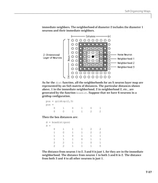
![7 Self-Organizing Networks
The link distance from one neuron is just the number of links, or steps, that
must be taken to get to the neuron under consideration. Thus if we calculate
the distances from the same set of neurons with linkdist we get:
dlink =
0 1 1 2 2 3
1 0 2 1 3 2
1 2 0 1 1 2
2 1 1 0 2 1
2 3 1 2 0 1
3 2 2 1 1 0
The Manhattan distance between two vectors x and y is calculated as:
D = sum(abs(x-y))
Thus if we have
W1 = [ 1 2; 3 4; 5 6]
W1 =
1 2
3 4
5 6
and
P1= [1;1]
P1 =
1
1
then we get for the distances
Z1 = mandist(W1,P1)
Z1 =
1
5
9
The distances calculated with mandist do indeed follow the mathematical
expression given above.
7-18](https://image.slidesharecdn.com/nnet-090922002848-phpapp01/85/Neural-Network-Toolbox-MATLAB-232-320.jpg)
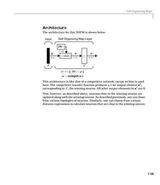
![7 Self-Organizing Networks
Creating a Self Organizing MAP Neural Network
(NEWSOM)
You can create a new SOFM network with the function newsom. This function
defines variables used in two phases of learning:
• Ordering phase learning rate
• Ordering phase steps
• Tuning phase learning rate
• Tuning phase neighborhood distance
These values are used for training and adapting.
Consider the following example.
Suppose that we wish to create a network having input vectors with two
elements that fall in the range 0 to 2 and 0 to 1 respectively. Further suppose
that we want to have six neurons in a hexagonal 2 by 3 network. The code to
obtain this network is:
net = newsom([0 2; 0 1] , [2 3]);
Suppose also that the vectors to train on are:
P = [.1 .3 1.2 1.1 1.8 1.7 .1 .3 1.2 1.1 1.8 1.7;...
0.2 0.1 0.3 0.1 0.3 0.2 1.8 1.8 1.9 1.9 1.7 1.8]
We can plot all of this with
plot(P(1,:),P(2,:),'.g','markersize',20)
hold on
plotsom(net.iw{1,1},net.layers{1}.distances)
hold off
7-20](https://image.slidesharecdn.com/nnet-090922002848-phpapp01/85/Neural-Network-Toolbox-MATLAB-234-320.jpg)
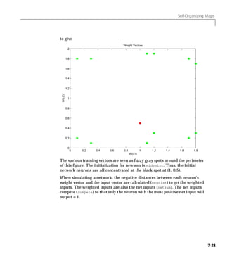
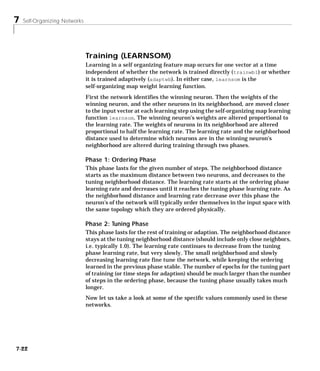
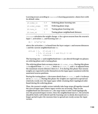
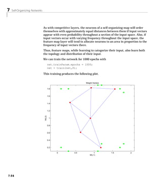
![Self-Organizing Maps
We can see that the neurons have started to move toward the various training
groups. Additional training will be required to get the neurons closer to the
various groups.
As noted previously, self-organizing maps differ from conventional competitive
learning in terms of which neurons get their weights updated. Instead of
updating only the winner, feature maps update the weights of the winner and
its neighbors. The result is that neighboring neurons tend to have similar
weight vectors and to be responsive to similar input vectors.
Examples
Two examples are described briefly below. You might try the demonstration
scripts demosm1 and demosm2 to see similar examples.
One-Dimensional Self-Organizing Map
Consider 100 two-element unit input vectors spread evenly between 0° and 90°.
angles = 0:0.5∗pi/99:0.5∗pi;
Here is a plot of the data
P = [sin(angles); cos(angles)];
1
0.8
0.6
0.4
0.2
0
0 0.5 1
7-25](https://image.slidesharecdn.com/nnet-090922002848-phpapp01/85/Neural-Network-Toolbox-MATLAB-239-320.jpg)
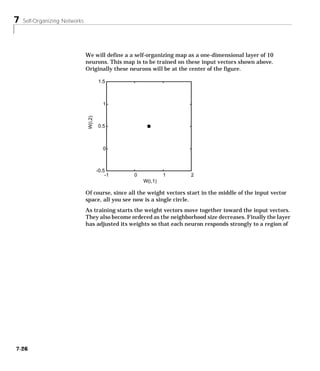
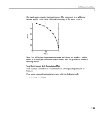
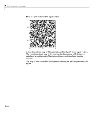
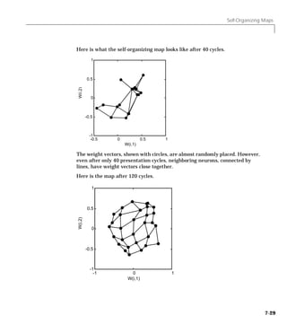
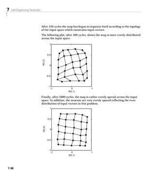

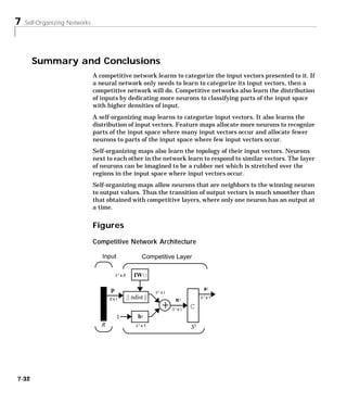
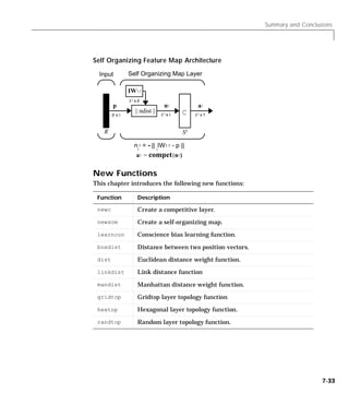


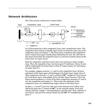

![Creating an LVQ Network (NEWLVQ)
Creating an LVQ Network (NEWLVQ)
An LVQ network can be created with the function newlvq.
net = newlvq(PR,S1,PC,LR,LF)
where
• PR is an Rx2 matrix of min and max values for R input elements,
• S1 is the number of first layer hidden neurons, and
• PC is an S2 element vector of typical class percentages.
The learning default is 0.01 and the default learning function is 'learnlv2'.
Suppose we have ten input vectors. We will create a network that assigns each
of these input vectors to one of four subclasses. Thus, we have four neurons in
the first competitive layer. These subclasses are then to be assigned to one of
two output classes by the two neurons in layer 2. The input vectors and targets
are specified by :
P = [-3 -2 -2 0 0 0 0 +2 + 2 +3; ...
0 +1 -1 +2 +1 -1 -2 +1 -1 0]
and
Tc = [1 1 1 2 2 2 2 1 1 1];
It may help to show the details of what we get from these two lines of code.
P =
-3 -2 -2 0 0 0 0 2 2 3
0 1 -1 2 1 -1 -2 1 -1 0
Tc =
1 1 1 2 2 2 2 1 1 1
8-5](https://image.slidesharecdn.com/nnet-090922002848-phpapp01/85/Neural-Network-Toolbox-MATLAB-253-320.jpg)
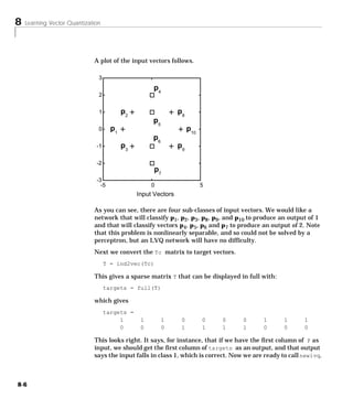
![Creating an LVQ Network (NEWLVQ)
We will call newlvq with the proper arguments so that it will create a network
with four neurons in the first layer and two neurons in the second layer. The
first layer weights will be initialized to the center of the input ranges with the
function midpoint. The second layer weights will have 60% (6 of the 10 in Tc
above) of its columns with a 1 in the first row, corresponding to class 1, and 40%
of its columns will have a 1 in the second row, corresponding to class 2.
net = newlvq(range(P),4,[.6 .4]);
We can check to see the initial values of the first layer weight matrix:
net.IW{1,1}
ans =
0 0
0 0
0 0
0 0
These zero weights are indeed the values at the midpoint of the range (-3 to +3)
of the inputs, as we would expect when using midpoint for initialization.
We can look at the second layer weights with
net.LW{2,1}
ans =
1 1 0 0
0 0 1 1
This makes sense too. It says that if the competitive layer produces a 1 as the
first or second element, the input vector will be classified as class 1. Otherwise
it will be in class 2.
You may notice that the first two competitive neurons are connected to the first
linear neuron (with weights of 1), while the second two competitive neurons are
connected to the second linear neuron. All other weights between the
competitive neurons and linear neurons have values of 0. Thus, each of the two
target classes (the linear neurons) is in fact, the union of two subclasses (the
competitive neurons).
8-7](https://image.slidesharecdn.com/nnet-090922002848-phpapp01/85/Neural-Network-Toolbox-MATLAB-255-320.jpg)

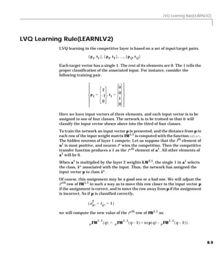

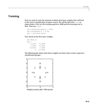
![8 Learning Vector Quantization
To check to see that these weights do indeed lead to the correct classification,
take the matrix P as input and simulate the network. Then see what
classifications are produced by the network.
Y = sim(net,P)
Yc = vec2ind(Y)
This gives
Yc =
1 1 1 2 2 2 2 1 1 1
which is what we expected. As a last check, try an input close to a vector that
was used in training.
pchk1 = [0; 0.5];
Y = sim(net,pchk1);
Yc1 = vec2ind(Y)
Which gives
Yc1 =
2
This looks right, for pchk1 is close to other vectors classified as 2. Similarly,
pchk2 = [1; 0];
Y = sim(net,pchk2);
Yc2 = vec2ind(Y)
gives
Yc2 =
1
This looks right too, for pchk2 is close to other vectors classified as 1s.
You might try demolvq1 to see an LVQ network problem.
Note that you get about the same results by running adapt for 100 epochs
through the10 vectors. This will give us 1000 vector presentations just the
same as was done when using train. First set the epochs to 100.
net.adaptparam.passes = 100;
8-12](https://image.slidesharecdn.com/nnet-090922002848-phpapp01/85/Neural-Network-Toolbox-MATLAB-260-320.jpg)
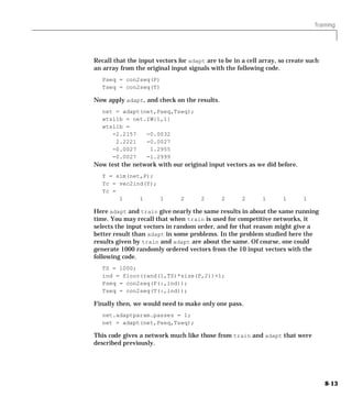
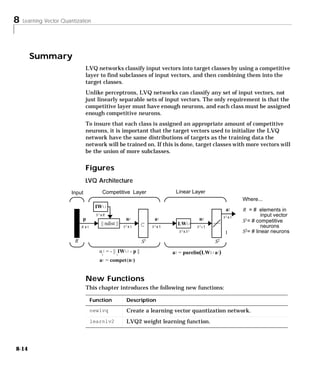

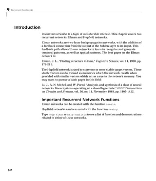
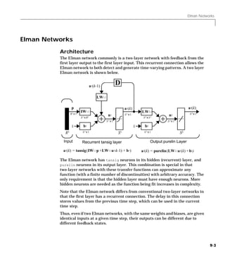
![9 Recurrent Networks
Because the network can store information for future reference it is able to
learn temporal patterns as well as spatial patterns. The Elman network can be
trained to respond to, and to generate, both kinds of patterns.
Creating an Elman Network (NEWELM)
An Elman network with two or more layers can be created with the function
newelm. The hidden layers commonly have tansig transfer functions, so that is
the default for newelm. As shown in the architecture diagram, purelin is
commonly the output layer transfer function.
The default backpropagation training function is trainbfg. One might use
trainlm, but it tends to proceed so rapidly that it does not necessarily do well
in the Elman network. The backprop weight/bias learning function default is
learngdm, and the default performance function is mse.
When the network is created, each layers weights and biases are initialized
with the Nguyen-Widrow layer initialization method implemented in the
function initnw.
Now consider an example. Suppose that we have a sequence of single element
input vectors in the range from 0 to 1. Suppose further that we want to have
five hidden layer tansig neurons and a single logsig output layer. The following
code creates the desired network.
net = newelm([0 1],[5 1],{'tansig','logsig'});
Simulation
Suppose that we would like to find the response of this network to an input
sequence of eight digits which are either 0 or 1.
P = round(rand(1,8))
P =
0 1 0 1 1 0 0 0
Recall that a sequence to be presented to a network is to be in cell array form.
We can convert P to this form with
Pseq = con2seq(P)
Pseq =
[0] [1] [0] [1] [1] [0] [0] [0]
9-4](https://image.slidesharecdn.com/nnet-090922002848-phpapp01/85/Neural-Network-Toolbox-MATLAB-266-320.jpg)
![Elman Networks
Now we can find the output of the network with the function sim.
Y = sim(net,Pseq)
Y =
Columns 1 through 5
[1.9875e-04] [0.1146] [5.0677e-05] [0.0017] [0.9544]
Columns 6 through 8
[0.0014] [5.7241e-05] [3.6413e-05]
We will convert this back to concurrent form with
z = seq2con(Y);
and can finally display the output in concurrent form with
z{1,1}
ans =
Columns 1 through 7
0.0002 0.1146 0.0001 0.0017 0.9544 0.0014 0.0001
Column 8
0.0000
Thus, once the network is created and the input specified, one need only
call sim.
9-5](https://image.slidesharecdn.com/nnet-090922002848-phpapp01/85/Neural-Network-Toolbox-MATLAB-267-320.jpg)
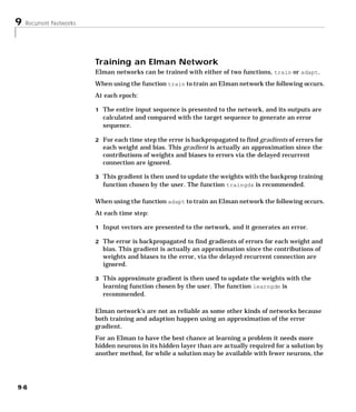
![Elman Networks
Elman network is less able to find the most appropriate weights for hidden
neurons since the error gradient is approximated. Therefore having a fair
number of neurons to begin with makes it more likely that the hidden neurons
will start out dividing up the input space in useful ways.
The function train trains an Elman network to generate a sequence of target
vectors when it is presented with a given sequence of input vectors. The input
vectors and target vectors are passed to train as matrices P and T. Train takes
these vectors and the initial weights and biases of the network, trains the
network using backpropagation with momentum and an adaptive learning
rate, and returns new weights and biases.
Let us continue with the example of the previous section, and suppose that we
wish to train a network with an input P and targets T as defined below.
P = round(rand(1,8))
P =
1 0 1 1 1 0 1 1
and
T = [0 (P(1:end-1)+P(2:end) == 2)]
T =
0 0 0 1 1 0 0 1
Here T is defined to be 0 except when two ones occur in P, in which case T will
be 1.
As noted previously, our network will have five hidden neurons in the first
layer.
net = newelm([0 1],[5 1],{'tansig','logsig'});
We will use trainbfg as the training function and train for 100 epochs. After
training we will simulate the network with the input P and calculate the
difference between the target output and the simulated network output.
net = train(net,Pseq,Tseq);
Y = sim(net,Pseq);
z = seq2con(Y);
z{1,1};
diff1 = T - z{1,1}
9-7](https://image.slidesharecdn.com/nnet-090922002848-phpapp01/85/Neural-Network-Toolbox-MATLAB-269-320.jpg)

![Hopfield Network
Hopfield Network
Fundamentals
The goal here is to design a network that stores a specific set of equilibrium
points such that, when an initial condition is provided, the network eventually
comes to rest at such a design point. The network is recursive in that the output
is fed back as the input once the network is in operation. Hopefully the network
output will settle on one of the original design points
The design method that we present is not perfect in that the designed network
may have undesired spurious equilibrium points in addition to the desired
ones. However, the number of these undesired points is made as small as
possible by the design method. Further, the domain of attraction of the
designed equilibrium points is as large as possible.
The design method is based on a system of first-order linear ordinary
differential equations that are defined on a closed hypercube of the state space.
The solutions exist on the boundary of the hypercube. These systems have the
basic structure of the Hopfield model but are easier to understand and design
than the Hopfield model.
The material in this section is based on the following paper: Jian-Hua Li,
Anthony N. Michel and Wolfgang Porod, “Analysis and synthesis of a class of
neural networks: linear systems operating on a closed hypercube,” IEEE
Trans. on Circuits and Systems vol 36, no. 11, pp. 1405-22, November 1989.
You may wish to read Chapter 18 of [HDB96] for further information on
Hopfield networks.
Architecture
The architecture of the network that we will use follows.
9-9](https://image.slidesharecdn.com/nnet-090922002848-phpapp01/85/Neural-Network-Toolbox-MATLAB-271-320.jpg)
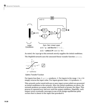
![Hopfield Network
Design(NEWHOP)
Li et. al. [LiMi89] have studied a system that has the basic structure of the
Hopfield network but is, in Li’s own words, “easier to analyze, synthesize and
implement than the Hopfield model.” The authors are enthusiastic about the
reference article, as it has many excellent points and is one of the most
readable in the field. However, the design is mathematically complex, and even
a short justification of it would burden this guide. Thus, we present the Li
design method, with thanks to Li et al., as a recipe that is found in the function
newhop.
Given a set of target equilibrium points represented as a matrix T of vectors,
newhop returns weights and biases for a recursive network. The network is
guaranteed to have stable equilibrium points at the target vectors, but it may
contain other spurious equilibrium points as well. The number of these
undesired points is made as small as possible by the design method.
Once the network has been designed, it can be tested with one or more input
vectors. Hopefully those input vectors close to target equilibrium points will
find their targets. As suggested by the network figure, an array of input vectors
may be presented at one time or in a batch. The network proceeds to give
output vectors which are fed back as inputs. These output vectors can be can
be compared to the target vectors to see how the solution is proceeding.
The ability to run batches of trial input vectors quickly allows you to check the
design in a relatively short time. First you might check to see that the target
equilibrium point vectors are indeed contained in the network. Then you could
try other input vectors to determine the domains of attraction of the target
equilibrium points and the locations of spurious equilibrium points if they are
present.
Consider the following design example. Suppose that we wish to design a
network with two stable points in a three dimensional space.
T = [-1 -1 1; 1 -1 1]'
T =
-1 1
-1 -1
1 1
We can execute the design with
net = newhop(T);
9-11](https://image.slidesharecdn.com/nnet-090922002848-phpapp01/85/Neural-Network-Toolbox-MATLAB-273-320.jpg)
![9 Recurrent Networks
Next we might check to make sure that the designed network is at these two
points. We can do this as follows. (Since Hopfield networks have no inputs, the
second argument to sim below is Q = 2 when using matrix notation).
Ai = T;
[Y,Pf,Af] = sim(net,2,[],Ai);
Y
This gives us
Y =
-1 1
-1 -1
1 1
Thus, the network has indeed been designed to be stable at its design points.
Next we might try another input condition that is not a design point, such as:
Ai = {[-0.9; -0.8; 0.7]}
which gives
Ai =
-0.9000
-0.8000
0.7000
.This point is reasonably close to the first design point, so one might anticipate
that the network would converge to that first point. To see if this happens, we
will run the following code. Note, incidentally, that we specified the original
point in cell array form. This allows us to run the network for more than one
step.
[Y,Pf,Af] = sim(net,{1 5},{},Ai);
Y{1}
We get
Y =
-1
-1
1
Thus, an original condition close to a design point did converge to that point.
9-12](https://image.slidesharecdn.com/nnet-090922002848-phpapp01/85/Neural-Network-Toolbox-MATLAB-274-320.jpg)
![Hopfield Network
This is, of course, our hope for all such inputs. Unfortunately, even the best
known Hopfield designs occasionally include undesired spurious stable points
that attract the solution.
Example
Consider a Hopfield network with just two neurons. Each neuron has a bias
and weights to accommodate two element input vectors weighted. We define
the target equilibrium points to be stored in the network as the two columns of
the matrix T.
T = [1 -1; -1 1]'
T =
1 -1
-1 1
Here is a plot of the Hopfield state space with the two stable points labeled
with ‘*’ markers.
Hopfield Network State Space
1
0.5
a(2
)
0
-0.5
-1
-1 0 1
a(1)
These target stable points are given to newhop to obtain weights and biases of
a Hopfield network.
net = newhop(T);
9-13](https://image.slidesharecdn.com/nnet-090922002848-phpapp01/85/Neural-Network-Toolbox-MATLAB-275-320.jpg)
![9 Recurrent Networks
The design returns a set of weights and a bias for each neuron. The results are
obtained from:
W= net.LW{1,1}
which gives
W =
0.6925 -0.4694
-0.4694 0.6925
and from
b = net.b{1,1}
which gives
b =
1.0e-16 *
0.6900
0.6900
Next the design is tested with the target vectors T to see if they are stored in
the network. The targets are used as inputs for the simulation function sim.
Ai = T;
[Y,Pf,Af] = sim(net,2,[],Ai);
Y =
1 -1
-1 1
As hoped, the new network outputs are the target vectors. The solution stays
at its initial conditions after a single update, and therefore will stay there for
any number of updates.
9-14](https://image.slidesharecdn.com/nnet-090922002848-phpapp01/85/Neural-Network-Toolbox-MATLAB-276-320.jpg)
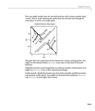
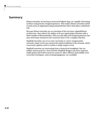
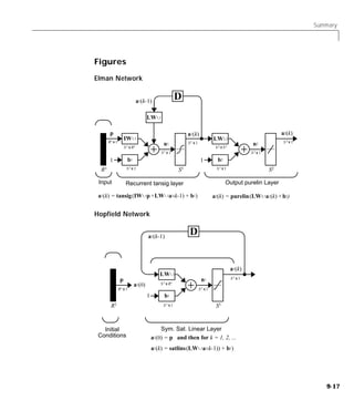
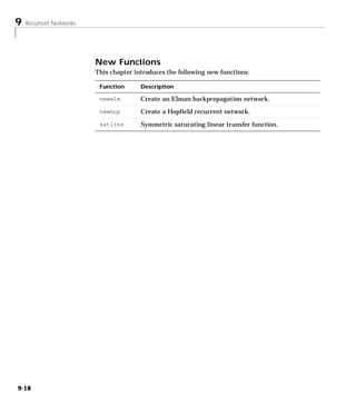
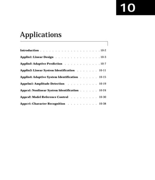
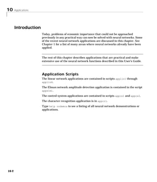
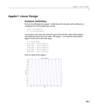
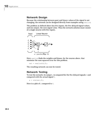
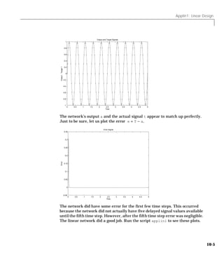

![Applin2: Adaptive Prediction
Applin2: Adaptive Prediction
In application script applin2, a linear network is trained incrementally with
adapt to predict a time series. Because the linear network is trained
incrementally, it can respond to changes in the relationship between past and
future values of the signal.
Problem Definition
The signal T to be predicted lasts six seconds with a sampling rate of 20
samples per second. However, after four seconds the signal’s frequency
suddenly doubles.
time1 = 0:0.05:4;
time2 = 4.05:0.024:6;
time = [time1 time2];
T = [sin(time1*4*pi) sin(time2*8*pi)];
Since we will be training the network incrementally, we will change t to a
sequence.
T = con2seq(T);
Here is a plot of this signal:
Signal to be Predicted
1
0.8
0.6
0.4
0.2
Target Signal
0
-0.2
-0.4
-0.6
-0.8
-1
0 1 2 3 4 5 6
Time
10-7](https://image.slidesharecdn.com/nnet-090922002848-phpapp01/85/Neural-Network-Toolbox-MATLAB-287-320.jpg)
![10 Applications
The input to the network is the same signal which makes up the target:
P = T;
Network Initialization
The network has only one neuron, as only one output value of the signal T is
being generated at each time step. This neuron has five inputs, the five delayed
values of the signal T.
Linear Layer
p(k) pd(k) a(k)
TDL W n(k)
1x1 5x1 1x1
1 1x3
2 1x1
3 1 b
4 1x1
5
The function newlin creates the network shown above. We will use a learning
rate of 0.1 for incremental training.
lr = 0.1;
delays = [1 2 3 4 5];
net = newlin(minmax(cat(2,P{:})),1,delays,lr);
[w,b] = initlin(P,t)
Network Training
The above neuron will be trained incrementally with adapt. Here is the code to
train the network on input/target signals P and T.
[net,a,e]=adapt(net,P,T);
Network Testing
Once the network has been adapted, we can plot its output signal and compare
it to the target signal.
10-8](https://image.slidesharecdn.com/nnet-090922002848-phpapp01/85/Neural-Network-Toolbox-MATLAB-288-320.jpg)
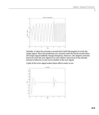

![Applin3: Linear System Identification
Applin3: Linear System Identification
Linear networks may be used to model real systems. If the real system is linear
or near linear then the linear network can act as a zero, or low, error model.
Problem Definition
Here is an input signal x which is given to a finite impulse response linear
system over a period of five seconds at 25 msec intervals.
time = 0:0.025:5;
X = sin(sin(time).*time*10);
Here is a plot of this input signal.
Input Signal to the System
1
0.8
0.6
0.4
0.2
Input Signal
0
-0.2
-0.4
-0.6
-0.8
-1
0 0.5 1 1.5 2 2.5 3 3.5 4 4.5 5
Time
Here are the measured outputs T of the system.
T = filter([1 0.5 –1.5],1,X);
Here is a plot of the systems output T.
10-11](https://image.slidesharecdn.com/nnet-090922002848-phpapp01/85/Neural-Network-Toolbox-MATLAB-291-320.jpg)
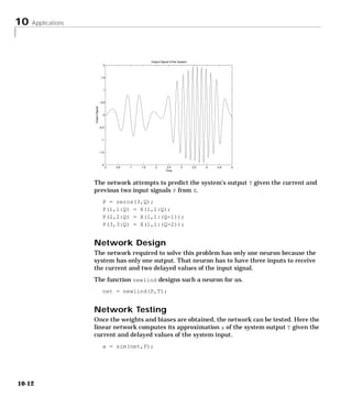
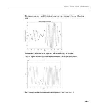
![Applin4: Adaptive System Identification
Applin4: Adaptive System Identification
Demonstration applin4 shows how to train a linear network to adaptively
model a linear system. By training the network incrementally, it can change its
behavior as the system it is modeling changes.
Problem Definition
Here is the input signal X to the system over a period of six seconds with a
sampling rate of 200 samples per second.
time1 = 0:0.005:4;
time2 = 4.005:0.005:6;
time = [time1 time2];
X = sin(sin(time*4).*time*8);
The input signal X to the system is plotted below.
Input Signal to System
1
0.8
0.6
0.4
0.2
Input Signal
0
-0.2
-0.4
-0.6
-0.8
-1
0 1 2 3 4 5 6
Time
Here is the output signal T of the system. Note that the system acts differently
in the intervals before and after the fourth second.
steps1 = length(time1);
[T1,state] = filter([1 –0.5],1,X(1:steps1));
steps2 = length(time2);
T2 = filter([0.9 –0.6],1,x((1:steps2) + steps1),state);
T = [T1 T2];
10-15](https://image.slidesharecdn.com/nnet-090922002848-phpapp01/85/Neural-Network-Toolbox-MATLAB-295-320.jpg)
![10 Applications
Here is a plot of the system’s outputs. Note that due to the complexity of the
signal, it is not apparent that the system changed at four seconds.
Output Signal of System
0.8
0.6
0.4
0.2
Output Signal
0
-0.2
-0.4
-0.6
-0.8
0 1 2 3 4 5 6
Time
The input to the network P is the system input signal X. The network must
estimate the system’s output T from the last two values of the input signal. We
need to convert the input and output to sequences, so that the training can be
done incrementally.
T = con2seq(T);
P = con2seq(X);
Network Initialization
The network is created with newlin, which generates the weights and biases
for the two-input linear neuron required for this problem. There will be a
tapped delay line with two delays at the input of the network. The last two
values of the input signal will be used to predict the system’s output.
lr = 0.5;
delays = [0 1];
net = newlin(minmax(cat(2,P{:})),1,delays,lr);
10-16](https://image.slidesharecdn.com/nnet-090922002848-phpapp01/85/Neural-Network-Toolbox-MATLAB-296-320.jpg)
![Applin4: Adaptive System Identification
Network Training
These weights and biases can now be trained incrementally on the signal with
adapt using the learning rate of 0.5, which was set by newlin.
[net,a,e]=adapt(net,P,T);
Network Testing
To see how well the network did, we could plot the network’s estimate a of the
system’s output against the actual output T. It turns out that the signals are
complex enough that this plot is not of much help. (You can run applin4 to
see it.)
Instead we can take a look at the error between the network output and the
system output. This plot is easier to interpret.
Error Signal
0.25
0.2
0.15
0.1
0.05
Error
0
-0.05
-0.1
-0.15
-0.2
-0.25
0 1 2 3 4 5 6
Time
The error plot shows that the network took 2.5 seconds to track the model with
a very high accuracy. Then at four seconds, when the system changed abruptly,
another 0.2 seconds were required for network to properly model it again.
Thoughts and Conclusions
Besides being interesting, an adaptive linear model of a system can be used to
obtain a great deal of information. For example, the adaptive model can be
analyzed at any given time to determine characteristics of the actual system.
10-17](https://image.slidesharecdn.com/nnet-090922002848-phpapp01/85/Neural-Network-Toolbox-MATLAB-297-320.jpg)
![Appelm1: Amplitude Detection
Appelm1: Amplitude Detection
Elman networks can be trained to recognize and produce both spatial and
temporal patterns. An example of a problem where temporal patterns are
recognized and classified with a spatial pattern is amplitude detection.
Amplitude detection requires that a wave form be presented to a network
through time, and that the network output the amplitude of the wave form.
This is not a difficult problem, but it demonstrates the Elman network design
process.
The following material describes code which is contained in the demonstration
script appelm1.
Problem Definition
The following code defines two sine wave forms, one with an amplitude of 1.0,
the other with an amplitude of 2.0:
p1 = sin(1:20);
p2 = sin(1:20)*2;
The target outputs for these wave forms will be their amplitudes.
t1 = ones(1,20);
t2 = ones(1,20)*2;
These wave forms can be combined into a sequence where each wave form
occurs twice. These longer wave forms will be used to train the Elman network.
p = [p1 p2 p1 p2];
t = [t1 t2 t1 t2];
We want the inputs and targets to be considered a sequence, so we need to
make the conversion from the matrix format.
Pseq = con2seq(p);
Tseq = con2seq(t);
10-19](https://image.slidesharecdn.com/nnet-090922002848-phpapp01/85/Neural-Network-Toolbox-MATLAB-299-320.jpg)
![10 Applications
Network Initialization
This problem requires that the Elman network detect a single value (the
signal), and output a single value (the amplitude), at each time step. Therefore
the network must have one input element, and one output neuron.
R = 1;% 1 input eleement
S2 = 1;% 1 layer 2 output neuron
The recurrent layer can have any number of neurons. However, as the
complexity of the problem grows, more neurons are needed in the recurrent
layer for the network to do a good job.
This problem is fairly simple, so only 10 recurrent neurons will be used in the
first layer.
S1 = 10;% 10 recurrent neurons in the first layer
Now the function newelm can be used to create initial weight matrices and bias
vectors for a network with one input which can vary between –2 and +2. We
will use variable learning rate (traingdx) for this example.
net = newelm([-2 2],[S1 S2],{'tansig','purelin'},'traingdx');
Network Training
Now call train.
[net,tr] = train(net,Pseq,Tseq);
As this function finishes training at 500 epochs, it displays the following plot
of errors.
10-20](https://image.slidesharecdn.com/nnet-090922002848-phpapp01/85/Neural-Network-Toolbox-MATLAB-300-320.jpg)
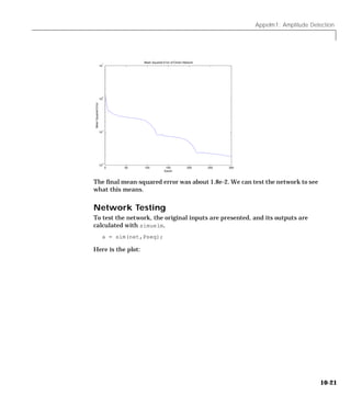
![10 Applications
Testing Amplitute Detection
2.2
2
1.8
Target - - Output ---
1.6
1.4
1.2
1
0.8
0 10 20 30 40 50 60 70 80
Time Step
The network does a good job. New wave amplitudes are detected with a few
samples. More neurons in the recurrent layer and longer training times would
result in even better performance.
The network has successfully learned to detect the amplitudes of incoming sine
waves.
Network Generalization
Of course, even if the network detects the amplitudes of the training wave
forms, it may not detect the amplitude of a sine wave with an amplitude it has
not seen before.
The following code defines a new wave form made up of two repetitions of a sine
wave with amplitude 1.6 and another with amplitude 1.2.
p3 = sin(1:20)*1.6;
t3 = ones(1,20)*1.6;
p4 = sin(1:20)*1.2;
t4 = ones(1,20)*1.2;
pg = [p3 p4 p3 p4];
tg = [t3 t4 t3 t4];
pgseq = con2seq(pg);
The input sequence pg and target sequence tg will be used to test the ability of
our network to generalize to new amplitudes.
10-22](https://image.slidesharecdn.com/nnet-090922002848-phpapp01/85/Neural-Network-Toolbox-MATLAB-302-320.jpg)
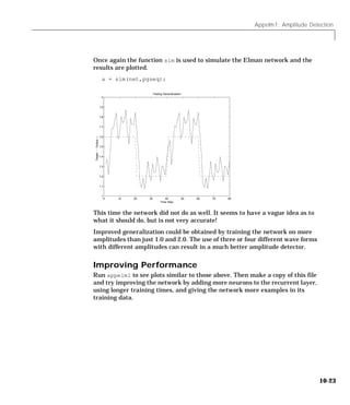
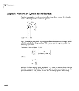
![Appcs1: Nonlinear System Identification
The inverted pendulum system is summarized with the function pmodel which
takes the current time t, pendulum angle, pendulum velocity, and the current,
and returns the derivatives of angle, velocity, and force.
x = [angle; vel; force];
dx = pmodel(t,x)
Because the current is an input to the system, its derivative is always returned
as 0.
We can simulate the pendulum from 0 to 0.05 seconds using ode23.
[time,X] = ode23(‘pmodel’,[0 0.05],x)
This function returns a row vector of times, and the matrix X of state vectors
associated with those times.
The problem is, given only the behavior of this pendulum, create a network
model that behaves in an identical manner.
Problem Definition
Examples of pendulum behavior must be created so that the network can be
trained. The following lines of code define several different pendulum angles,
pendulum velocities, and forces.
deg2rad = pi/180;
angle = [–20:40:200]*deg2rad;
vel = [–90:36:90]*deg2rad;
force = –30:6:30;
By taking all possible combinations of these values, and also a set of steady
state conditions at various angles, we get a matrix Pm of 749 pendulum state/
input conditions, where the pendulum’s state is its angle and velocity, and its
input is the current.
angle2 = [-20:10:200]*deg2rad;
Pm = [combvec(angle,vel,force);
[angle2; zeros(2,length(angle2))]];
Next each of these 749 initial state/input conditions are applied to the
pendulum, and its next state, 0.05 seconds later is measured. The next state
consists of the pendulum angle and velocity after 0.05 seconds. The result is a
matrix Tm of the 749 2-element next states. (Actually, we will use the difference
10-25](https://image.slidesharecdn.com/nnet-090922002848-phpapp01/85/Neural-Network-Toolbox-MATLAB-305-320.jpg)
![10 Applications
between the next state and the current state as the target. The neural network
model will learn to predict the change in state over 0.05 seconds. This is done
because the state does not change by a large amount in this period of time, and
we can improve the performance of the model if we predict only the change in
state. If we need to know the actual state we simply need to add the change to
the previous state.)
Network Initialization
The network must transform the pendulum state and input into a next state
(or change in state). As there are two states (angle and velocity) and one input,
the network requires three inputs and one output.
The function initff is used to create a two-layer tansig/purelin network with
these number of inputs and outputs and eight hidden neurons.
S1 = 8;
[S2,Q] = size(Tm);
mnet = newff(minmax(Pm),[S1 S2],{'tansig' 'purelin'},'trainlm');
We use this network to model the nonlinear pendulum system.
Network Training
The Levenberg-Marquardt training function trainlm is used to obtain a
solution in the minimum amount of time. The network is trained for up to 500
epochs, displaying progress every epoch, and with a typical error of 0.0037
radians (0.25 degrees) for the 749 training vectors and the network’s two
outputs.
mnet.trainParam.goal = (0.0037^2);
mnet = train(mnet,Pm,Tm);
Network Testing
The network is tested by simulating its response for the following initial
conditions and comparing the results to the pendulum response.
angle = 5*deg2rad;
vel = 0*deg2rad;
force = 0;
x = [angle; vel; force];
10-26](https://image.slidesharecdn.com/nnet-090922002848-phpapp01/85/Neural-Network-Toolbox-MATLAB-306-320.jpg)
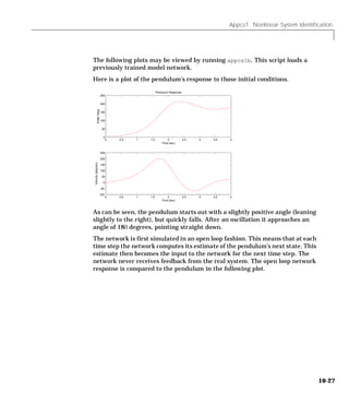
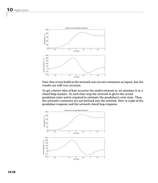
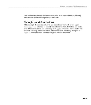
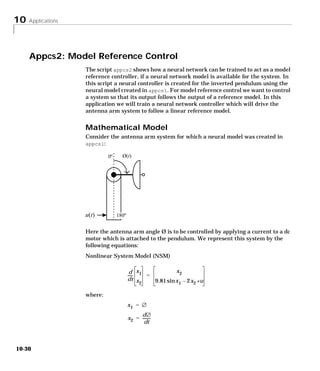
![Appcs2: Model Reference Control
and u is the force applied to the pendulum by a motor. A positive force turns
the pendulum clockwise. The 9.81sin x1 term is the force of gravity on the
pendulum and the –2x2 term is viscous friction acting against the velocity.
Suppose that we would like the closed loop system to respond with the
dynamics given by the Linear Reference Model (LRM).
d x x2
---- 1 =
- + 0
dt x – 9x 1 – 6x 2 9r
2
where r is the desired output angle.
Now let us train a neural network to help perform this model reference control.
Neural Design
A neural controller can be created for the case where the mathematical model
is not available. All that is required is a neural model of the original system
(which is created in appcs1) and a model of our desired system.
The desired linear reference model, described mathematically above, is
available in the function plinear. It takes the current time t, pendulum angle,
pendulum velocity, and the demand angle, and returns the derivatives of angle,
velocity, and demand.
x = [angle; vel; demand];
dx = pmodel(t,x)
Because the demand is an input to the system, its derivative is always returned as 0.
We can simulate the desired linear reference model from 0 to 0.05 seconds
using ode23.
[time,X] = ode23('plinear',0,0.05,x)
This function returns a row vector of times, and the matrix X of state vectors
associated with those times.
We would like to find a controller network which takes the current pendulum
angle, velocity, and the demand angle as inputs, and outputs a current which
can be applied to the pendulum. This current value should make the
pendulum’s next state (in 0.05 seconds) identical to that defined by the desired
linear reference model.
10-31](https://image.slidesharecdn.com/nnet-090922002848-phpapp01/85/Neural-Network-Toolbox-MATLAB-311-320.jpg)
![10 Applications
Problem Definition
Before the controller can be trained, examples of initial states and desired next
states must be created.
The following lines of code define several different pendulum angles, pendulum
velocities, and demand angles.
deg2rad = pi/180;
angle = [–200:40:200]*deg2rad;
vel = [–90:36:90]*deg2rad;
demand = –180:40:180*deg2rad;
By taking all possible combinations of these values in addition to a set of steady
state initial conditions (velocity = 0, demand = angle) we get a matrix P of 381
pendulum state/input conditions, where the pendulum’s state is its angle and
velocity, and its input is the current.
angle2 = [-10:10:190]*deg2rad;
Pc = [combvec(anglevel,demand)
[angle2; angle2*0; angle2]];
Next each of these 381 initial state/input conditions are applied to the desired
linear model, and its next state, 0.05 seconds later is measured. The next state
consists of the desired pendulum angle and velocity after 0.05 seconds. The
result is a matrix Tc of the 381 two-element target next states. (As in the
identification problem appcs1, we will actually use the difference between the
next state and the current state as the target. The neural network model
learned to predict the change in state over 0.05 seconds. This was done because
the state does not change by a large amount in this period of time, and we can
improve the performance of the model if we predict only the change in state. If
we need to know the actual state we simply need to add the change to the
previous state.)
Network Initialization
The neural controller, like the neural pendulum model, is a
tansig/purelin network. Here newff creates such a network for the controller
which will have eight hidden neurons, and one output (the current to the
pendulum).
S1 = 8;
cnet = newff(minmax(Pc),[S1 1],{'tansig' 'purelin'});
10-32](https://image.slidesharecdn.com/nnet-090922002848-phpapp01/85/Neural-Network-Toolbox-MATLAB-312-320.jpg)
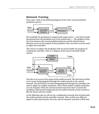
![10 Applications
layers. (The following code uses advanced features of the Neural Network
Toolbox. You may want to look through Chapter 11 and Chapter 12 before
reviewing the rest of this application.)
numInputs = 2;
numLayers = 4;
tnet = network(numInputs,numLayers);
We next need to set up the network connections.
tnet.biasConnect = [1 1 1 1]';
tnet.inputConnect = [1 0 1 0; 1 0 0 0]';
tnet.layerConnect = [0 0 0 0; 1 0 0 0; 0 1 0 0; 0 0 1 0];
tnet.outputConnect = [0 0 0 1];
tnet.targetConnect = [0 0 0 1];
Now we define the input and layer parameters. The first input corresponds to
the states, and the second input is the demand.
tnet.inputs{1}.range = minmax(Pc(1:2,:));
tnet.inputs{2}.range = minmax(Pc(3,:));
Next we define the size of each layer and the transfer functions.
tnet.layers{1}.size = S1;
tnet.layers{1}.transferFcn = 'tansig';
tnet.layers{2}.size = 1;
tnet.layers{2}.transferFcn = 'purelin';
tnet.layers{3}.size = 8;
tnet.layers{3}.transferFcn = 'tansig';
tnet.layers{4}.size = 2;
tnet.layers{4}.transferFcn = 'purelin';
We will use the quasi-Newton training function trainbfg to train the network
to minimize the mean square error.
tnet.performFcn = 'mse';
tnet.trainFcn = 'trainbfg';
10-34](https://image.slidesharecdn.com/nnet-090922002848-phpapp01/85/Neural-Network-Toolbox-MATLAB-314-320.jpg)
![Appcs2: Model Reference Control
We now set the initial weights and biases in the total network that correspond
to the controller network. These will be adjusted during the training process,
so the learn parameter is set to 1.
tnet.IW{1,1} = cnet.IW{1,1}(:,1:2);
tnet.inputWeights{1,1}.learn = 1;
tnet.IW{1,2} = cnet.IW{1,1}(:,3);
tnet.inputWeights{1,2}.learn = 1;
tnet.b{1} = cnet.b{1};
tnet.biases{1}.learn = 1;
tnet.b{2} = cnet.b{2};
tnet.biases{2}.learn = 1;
tnet.LW{2,1} = cnet.LW{2,1};
tnet.layerWeights{2,1}.learn = 1;
Finally, we set the weights and biases in the total network that correspond to
the model network. These will not be adjusted during the training process, so
the learn parameter is set to 0.
tnet.IW{3,1} = mnet.IW{1,1}(:,1:2);
tnet.inputWeights{3,1}.learn = 0;
tnet.LW{3,2} = mnet.IW{1,1}(:,3);
tnet.layerWeights{3,2}.learn = 0;
tnet.b{3} = mnet.b{1};
tnet.biases{3}.learn = 0;
tnet.LW{4,3} = mnet.LW{2,1};
tnet.layerWeights{4,3}.learn = 0;
tnet.b{4} = mnet.b{2};
tnet.biases{4}.learn = 0;
Here train is called to do this training for us. The controller will be trained for
up to 600 epochs, displaying progress every 5 epochs, to a typical error of 0.002
radians (0.11 degrees) for each of the 381 training vectors for each of the 2
model network outputs.
tnet.trainParam.show = 5;
tnet.trainParam.epochs = 600;
tnet.trainParam.goal = (0.002^2);
[tnet,tr] = train(tnet,{Pc(1:2,:); Pc(3,:)},{Tc});
The network contains the weights and biases of both the controller and model
networks, but the model weights do not change. Only the controller weights are
10-35](https://image.slidesharecdn.com/nnet-090922002848-phpapp01/85/Neural-Network-Toolbox-MATLAB-315-320.jpg)
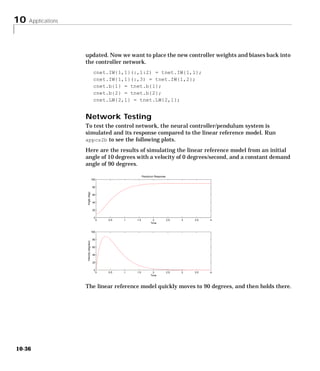
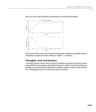
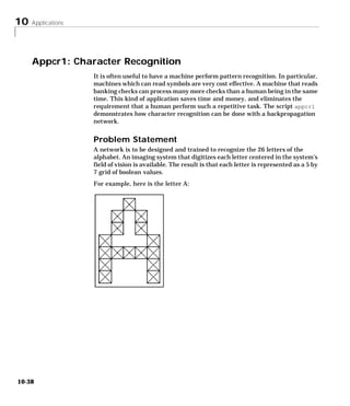
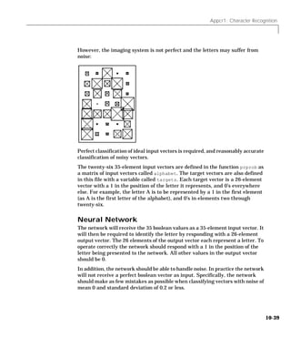
![10 Applications
Architecture
The neural network needs 35 inputs and 26 neurons in its output layer to
identify the letters. The network is a two-layer log-sigmoid/log-sigmoid
network. The log-sigmoid transfer function was picked because its output
range (0 to 1) is perfect for learning to output boolean values.
Input Hidden Layer Output Layer
p1 a1 a2
35 x 1
IW1,1 10 x 1
LW2,1 26 x 1
10 x 35
n1 26 x 10
n2
10 26 x 1
x1
1 b1 1 b2
35 10 x 1 10 26 x 1 26
a1 = logsig (IW1,1p1 +b1) a2 = logsig(LW2,1a1 +b2)
The hidden (first) layer has 10 neurons. This number was picked by guesswork
and experience. If the network has trouble learning, then neurons can be added
to this layer.
The network is trained to output a 1 in the correct position of the output vector
and to fill the rest of the output vector with 0’s. However, noisy input vectors
may result in the network not creating perfect 1’s and 0’s. After the network
has been trained the output will be passed through the competitive transfer
function compet. This makes sure that the output corresponding to the letter
most like the noisy input vector takes on a value of 1 and all others have a value
of 0. The result of this post-processing is the output that is actually used.
Initialization
The two layer network is created with newff.
S1 = 10; S2 = 26;
net = newff(minmax(P),[S1 S2],{'logsig' 'logsig'},'traingdx');
Training
To create a network that can handle noisy input vectors it is best to train the
network on both ideal and noisy vectors. To do this the network will first be
trained on ideal vectors until it has a low sum-squared error.
10-40](https://image.slidesharecdn.com/nnet-090922002848-phpapp01/85/Neural-Network-Toolbox-MATLAB-320-320.jpg)
![Appcr1: Character Recognition
Then the network will be trained on 10 sets of ideal and noisy vectors. The
network is trained on two copies of the noise-free alphabet at the same time as
it is trained on noisy vectors. The two copies of the noise-free alphabet are used
to maintain the network’s ability to classify ideal input vectors.
Unfortunately, after the training described above the network may have
learned to classify some difficult noisy vectors at the expense of properly
classifying a noise free vector. Therefore, the network will again be trained on
just ideal vectors. This ensures that the network will respond perfectly when
presented with an ideal letter.
All training is done using backpropagation with both adaptive learning rate
and momentum with the function trainbpx.
Training Without Noise
The network is initially trained without noise for a maximum of 5000 epochs
or until the network sum-squared error falls beneath 0.1.
P = alphabet;
T = targets;
net.performFcn = 'sse';
net.trainParam.goal = 0.1;
net.trainParam.show = 20;
net.trainParam.epochs = 5000;
net.trainParam.mc = 0.95;
[net,tr] = train(net,P,T);
Training With Noise
To obtain a network not sensitive to noise, we trained with two ideal copies and
two noisy copies of the vectors in alphabet. The target vectors consist of four
copies of the vectors in target. The noisy vectors have noise of mean 0.1 and
0.2 added to them. This forces the neuron to learn how to properly identify
noisy letters, while requiring that it can still respond well to ideal vectors.
10-41](https://image.slidesharecdn.com/nnet-090922002848-phpapp01/85/Neural-Network-Toolbox-MATLAB-321-320.jpg)
![10 Applications
To train with noise the maximum number of epochs is reduced to 300 and the
error goal is increased to 0.6, reflecting that higher error is expected due to
more vectors, including some with noise, are being presented.
netn = net;
netn.trainParam.goal = 0.6;
netn.trainParam.epochs = 300;
T = [targets targets targets targets];
for pass = 1:10
P = [alphabet, alphabet, ...
(alphabet + randn(R,Q)*0.1), ...
(alphabet + randn(R,Q)*0.2)];
[netn,tr] = train(netn,P,T);
end
Training Without Noise Again
Once the network has been trained with noise it makes sense to train it without
noise once more to ensure that ideal input vectors are always classified
correctly. Therefore the network is again trained with code identical to the
"Training Without Noise" section.
System Performance
The reliability of the neural network pattern recognition system is measured
by testing the network with hundreds of input vectors with varying quantities
of noise. The script file appcr1 tests the network at various noise levels and
then graphs the percentage of network errors vs. noise. Noise with mean of 0
and standard deviation from 0 to 0.5 are added to input vectors. At each noise
level 100 presentations of different noisy versions of each letter are made and
the network’s output is calculated. The output is then passed through the
competitive transfer function so that only one of the 26 outputs, representing
the letters of the alphabet, has a value of 1.
10-42](https://image.slidesharecdn.com/nnet-090922002848-phpapp01/85/Neural-Network-Toolbox-MATLAB-322-320.jpg)
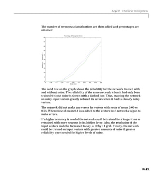
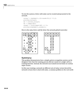
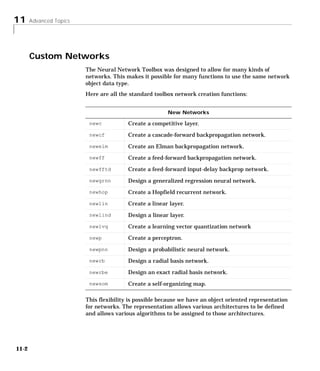

![11 Advanced Topics
Custom Network
Before you can build a network you need to know what it looks like. For
dramatic purposes (and to give the toolbox a work out) this section will lead you
through the creation of the wild and complicated network shown below.
Inputs Layers 1 and 2 Layer 3 Outputs
p1(k)
IW1,1
2x1 TDL
n1(k) 1 LW3,3
4x2
4x1 1 x (1*1)
1 b1 a1(k)
LW3,1
IW3,1
4x1
2 4x1 4 1x4
n3(k) a3(k) y2(k)
1x1 1x1 1x1
a1(k) = tansig (IW1,1p1(k) +b1) 1 b3
1x1
a2(k) 1
TDL IW2,1 LW3,2
0,1 3x1
n2(k) 1x3 y1(k)
3 x (2*2)
3x1 3x1
p2(k)
TDL IW2,2
5x1 1
5 3 x (1*5) 3
a2(k) = logsig (IW2,1 [p1(k);p1(k-1) ]+ IW2,2p2(k-1)) a3(k)=purelin(LW3,3a3(k-1)+IW3,1 a1 (k)+b3+LW3,2a2 (k))
Each of the two elements of the first network input is to accept values ranging
between 0 and 10. Each of the five elements of the second network input will
range from -2 to 2.
Before you can complete your design of this network, the algorithms it employs
for initialization and training must be specified.
We will agree here that each layer’s weights and biases will be initialized with
the Nguyen-Widrow layer initialization method (initnw). Also, the network is
to be trained with the Levenberg-Marquardt backpropagation (trainlm), so
that, given example input vectors, the outputs of the third layer will learn to
match the associated target vectors with minimal mean squared error (mse).
11-4](https://image.slidesharecdn.com/nnet-090922002848-phpapp01/85/Neural-Network-Toolbox-MATLAB-328-320.jpg)
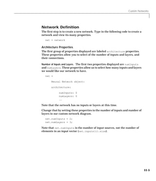
![11 Advanced Topics
Bias Connections. Type net and hit return to view its properties again. The
network now has two inputs and three layers.
net =
Neural Network object:
architecture:
numInputs: 2
numLayers: 3
Now look at the next five properties.
biasConnect: [0; 0; 0]
inputConnect: [0 0; 0 0; 0 0]
layerConnect: [0 0 0; 0 0 0; 0 0 0]
outputConnect: [0 0 0]
targetConnect: [0 0 0]
These matrices of 1’s and 0’s represent the presence or absence of bias, input
weight, layer weight, output, and target connections. They are currently all
zeros indicating that the network does not have any such connections.
Note that the bias connection matrix is a 3 × 1 vector. To create a bias
connection to the ith layer you can set net.biasConnect(i) to 1. Specify that
the first and third layer’s are to have bias connections, as our wacky diagram
indicates, by typing in the following code.
net.biasConnect(1) = 1;
net.biasConnect(3) = 1;
Note that you could also define those connections with a single line of code.
net.biasConnect = [1; 0; 1];
Input and Layer Weight Connections. The input connection matrix is 3 × 2 ,
representing the presence of connections from 2 sources (the two inputs) to 3
destinations (the three layers). Thus net.inputConnect(i,j) represents the
presence of an input weight connection going to the ith layer from the jth input.
11-6](https://image.slidesharecdn.com/nnet-090922002848-phpapp01/85/Neural-Network-Toolbox-MATLAB-330-320.jpg)
![Custom Networks
Connect the first input to the first and second layers, and the second input to
the second layer (as is indicated by the custom network diagram) by typing in
the following three lines of code,
net.inputConnect(1,1) = 1;
net.inputConnect(2,1) = 1;
net.inputConnect(2,2) = 1;
or this single line of code:
net.inputConnect = [1 0; 1 1; 0 0];
Similarly, net.layerConnect(i.j) represents the presence of a layer weight
connection going to the ith layer from the jth layer. Connect layers 1, 2 and 3
to layer 3 as follows.
net.layerConnect = [0 0 0; 0 0 0; 1 1 1];
Output and Target Connections. Both the output and target connection matrices
are 1 × 3 matrices, indicating that they connect to one destination (the
external world) from three sources (the three layers).
Connect layers 2 and 3 to network outputs with this line of code.
net.outputConnect = [0 1 1];
Type another line of code to give layer 3 a target connection.
net.targetConnect = [0 0 1];
The layer 3 target will be compared to the output of layer 3 to generate an error
to be used when measuring the performance of the network, or when updating
the network during training or adaption.
Number of Outputs and Targets
Type net and hit Enter to view the updated properties. The final four
architecture properties are read-only values, which means their values are
determined by the choices we make for other properties. The first two read-only
properties have the following values.
numOutputs: 2 (read-only)
numTargets: 1 (read-only)
11-7](https://image.slidesharecdn.com/nnet-090922002848-phpapp01/85/Neural-Network-Toolbox-MATLAB-331-320.jpg)
![11 Advanced Topics
By defining output connections from layers 2 and 3, and a target connection
from layer 3, you have specified that the network has two outputs and one
target.
Subobject Properties
The next group of properties are as follows.
subobject structures:
inputs: {2x1 cell} of inputs
layers: {3x1 cell} of layers
outputs: {1x3 cell} containing 2 outputs
targets: {1x3 cell} containing 1 target
biases: {3x1 cell} containing 2 biases
inputWeights: {3x2 cell} containing 3 input weights
layerWeights: {3x3 cell} containing 3 layer weights
Inputs
When you set the number of inputs (net.numInputs) to 2, the inputs property
became a cell array of two input structures. Each ith input structure
(net.inputs{i}) contains addition properties associated with the ith input.
Type this line of code to see how the input structures are arranged.
net.inputs
ans =
[1x1 struct]
[1x1 struct]
Type the following line of code to see the properties associated with the first
input.
net.inputs{1}
The properties should appear as follows.
ans =
range: [0 1]
size: 1
userdata: [1x1 struct]
11-8](https://image.slidesharecdn.com/nnet-090922002848-phpapp01/85/Neural-Network-Toolbox-MATLAB-332-320.jpg)
![Custom Networks
Note that the range property only has one row. This indicates that the input
has only one element, which varies from 0 to 1. The size property also
indicates that this input has just 1 element.
The first input vector of the custom network is to have two elements ranging
from 0 to 10. Specify this by altering the range property of the first input as
follows.
net.inputs{1}.range = [0 10; 0 10];
If we examine the first input’s structure again, we will see that it now has the
correct size which was inferred from the new range values.
ans =
range: [2x2 double]
size: 2
userdata: [1x1 struct]
Set the second inputs ranges to be from -2 to 2 for five elements as follows.
net.inputs{2}.range = [-2 2; -2 2; -2 2; -2 2; -2 2];
Layers . When we set the number of layers (net.numLayers) to 3, the layers
property became a cell array of three layer structures. Type the following line
of code to see the properties associated with the first layer.
net.layers{1}
ans =
dimensions: 1
distanceFcn: 'dist'
distances: 0
initFcn: 'initwb'
netInputFcn: 'netsum'
positions: 0
size: 1
topologyFcn: 'hextop'
transferFcn: 'purelin'
userdata: [1x1 struct]
11-9](https://image.slidesharecdn.com/nnet-090922002848-phpapp01/85/Neural-Network-Toolbox-MATLAB-333-320.jpg)
![11 Advanced Topics
Type the following three lines of code to change the first layer’s size to 4
neurons, its transfer function to tansig, and its initialization function to the
Nguyen-Widrow function as required for the custom network diagram.
net.layers{1}.size = 4;
net.layers{1}.transferFcn = ’tansig’;
net.layers{1}.initFcn = ’initnw’;
The second layer is to have 3 neurons, the logsig transfer function, and be
initialized with initnw. Thus, set the second layer’s properties to the desired
values as follows.
net.layers{2}.size = 3;
net.layers{2}.transferFcn = ’logsig’;
net.layers{2}.initFcn = ’initnw’;
The third layer’s size and transfer function properties don’t need to be changed
since the defaults match those shown in the network diagram. You only need
to set its initialization function as follows.
net.layers{3}.initFcn = ’initnw’;
Output and Targets. Take a look at how the outputs property is arranged with
this line of code.
net.outputs
ans =
[] [1x1 struct] [1x1 struct]
Note that outputs contains two output structures, one for layer 2 and one for
layer 3. This arrangement occurred automatically when net.outputConnect
was set to [0 1 1].
View the second layer’s output structure with the following expression.
net.outputs{2}
ans =
size: 3
userdata: [1x1 struct]
The size was automatically set to 3 when the second layer’s size
(net.layers{2}.size) was set to that value. Take a look at the third layer’s
output structure if you want to verify that it also has the correct size.
11-10](https://image.slidesharecdn.com/nnet-090922002848-phpapp01/85/Neural-Network-Toolbox-MATLAB-334-320.jpg)
![Custom Networks
Similarly, targets contains one structure representing the third layer’s target.
Type these two lines of code to see how targets is arranged and to view the
third layer’s target properties.
net.targets
ans =
[] [] [1x1 struct]
net.targets{3}
ans =
size: 1
userdata: [1x1 struct]
Biases, Input Weights and Layer Weights. Enter the following lines of code to see how
bias and weight structures are arranged.
net.biases
net.inputWeights
net.layerWeights
Here are the results for typing net.biases:
ans =
[1x1 struct]
[]
[1x1 struct]
If you examine the results you will note that each contains a structure where
the corresponding connections (net.biasConnect, net.inputConnect, and
net.layerConnect) contain a 1.
Take a look at their structures with these lines of code.
net.biases{1}
net.biases{3}
net.inputWeights{1,1}
net.inputWeights{2,1}
net.inputWeights{2,2}
net.layerWeights{3,1}
net.layerWeights{3,2}
net.layerWeights{3,3}
11-11](https://image.slidesharecdn.com/nnet-090922002848-phpapp01/85/Neural-Network-Toolbox-MATLAB-335-320.jpg)
![11 Advanced Topics
For example, typing net.biases{1} results in the following output:
ans =
initFcn: ''
learn: 1
learnFcn: ''
learnParam: ''
size: 4
userdata: [1x1 struct]
Specify the weights tap delay lines in accordance with the network diagram, by
setting each weights delays property.
net.inputWeights{2,1}.delays = [0 1];
net.inputWeights{2,2}.delays = 1;
net.layerWeights{3,3}.delays = 1;
Network Functions
Type net and press return again to see the next set of properties.
functions:
adaptFcn: (none)
initFcn: (none)
performFcn: (none)
trainFcn: (none)
Each of these properties defines a function for a basic network operation.
Set the initialization function to initlay so the network will initialize itself
according to the layer initialization functions which we have already set to
initnw the Nguyen-Widrow initialization function.
net.initFcn = 'initlay';
This meets the initialization requirement of our network.
Set the performance function to mse (mean squared error) and the training
function to trainlm (Levenberg-Marquardt backpropagation) to meet the final
requirement of the custom network.
net.performFcn = 'mse';
net.trainFcn = 'trainlm';
11-12](https://image.slidesharecdn.com/nnet-090922002848-phpapp01/85/Neural-Network-Toolbox-MATLAB-336-320.jpg)
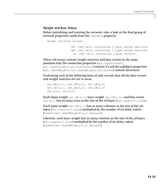
![11 Advanced Topics
Network Behavior
Initialization
Initialize your network with the following line of code.
net = init(net)
Reference the network’s biases and weights again to see how they have
changed.
net.IW{1,1}, net.IW{2,1}, net.IW{2,2}
net.IW{3,1}, net.LW{3,2}, net.LW{3,3}
net.b{1}, net.b{3}
For example:
net.IW{1,1}
ans =
-0.3040 0.4703
-0.5423 -0.1395
0.5567 0.0604
0.2667 0.4924
Training
Define the following cell array of two input vectors (one with two elements, one
with five) for two time steps (i.e. two columns).
P = {[0; 0] [2; 0.5]; [2; -2; 1; 0; 1] [-1; -1; 1; 0; 1]}
We would like the network to respond with the following target sequence.
T = {1 -1}
Before training we can simulate the network to see whether the initial
network’s response Y is close to the target T.
Y = sim(net,P)
Y =
[3x1 double] [3x1 double]
[ 0.0456] [ 0.2119]
11-14](https://image.slidesharecdn.com/nnet-090922002848-phpapp01/85/Neural-Network-Toolbox-MATLAB-338-320.jpg)
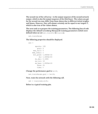
![11 Advanced Topics
Performance is 3.91852e-16, Goal is 1e-10
5
10
0
10
Training-Blue Goal-Black
-5
10
-10
10
-15
10
-20
10
0 0.5 1 1.5 2 2.5 3 3.5 4
4 Epochs
After training you can simulate the network to see if it has learned to respond
correctly.
Y = sim(net,P)
Y =
[3x1 double] [3x1 double]
[ 1.0000] [ -1.0000]
Note that the second network output (i.e. the second row of the cell array Y),
which is also the third layer’s output, does match the target sequence T.
11-16](https://image.slidesharecdn.com/nnet-090922002848-phpapp01/85/Neural-Network-Toolbox-MATLAB-340-320.jpg)
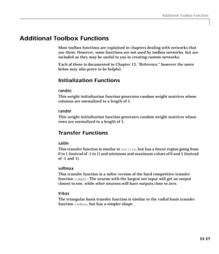

![11 Advanced Topics
Simulation Functions
You can create three kinds of simulation functions: transfer, net input, and
weight functions. You can also provide associated derivative functions to
enable backpropagation learning with your functions.
Transfer Functions
Transfer functions calculate a layer’s output vector (or matrix) A given its net
input vector (or matrix) N. The only constraint on the relationship between the
output and net input is that the output must have the same dimensions as the
input.
Once defined you can assign your transfer function to any layer of a network.
For example, the following line of code assigns the transfer function yourtf to
the second layer of a network.
net.layers{2}.transferFcn = 'yourtf';
Your transfer function will then be used whenever you simulate your network.
[Y,Pf,Af] = sim(net,P,Pi,Ai)
To be a valid transfer function your function must calculate outputs A from net
inputs N as follows,
A = yourtf(N)
where:
• N is an SxQ matrix of Q net input (column) vectors.
• A is an SxQ matrix of Q output (column) vectors.
Your transfer function must also provide information about itself using this
calling format,
info = yourtf(code)
where the correct information is returned for each of the following string codes:
• 'version' - Returns the Neural Network Toolbox version (3.0).
• 'deriv' - Returns the name of the associated derivative function.
• 'output' - Returns the output range.
• 'active' - Returns the active input range.
11-20](https://image.slidesharecdn.com/nnet-090922002848-phpapp01/85/Neural-Network-Toolbox-MATLAB-344-320.jpg)
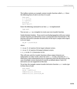
![11 Advanced Topics
Use this command to see how mydtf was implemented.
type mydtf
You can use mydtf as a template to create your own transfer derivative
functions.
Net Input Functions
Net input functions calculate a layer’s net input vector (or matrix) N given its
weighted input vectors (or matrices) Zi. The only constraints on the
relationship between the net input and the weighted inputs are that the net
input must have the same dimensions as the weighted inputs, and that the
function cannot be sensitive to the order of the weight inputs.
Once defined you can assign your net input function to any layer of a network.
For example, the following line of code assigns the transfer function yournif to
the second layer of a network.
net.layers{2}.netInputFcn = 'yournif';
Your net input function will then be used whenever you simulate your network.
[Y,Pf,Af] = sim(net,P,Pi,Ai)
To be a valid net input function your function must calculate outputs A from
net inputs N as follows,
N = yournif(Z1,Z2,...)
where:
• Zi is the ith S × Q matrix of Q weighted input (column) vectors.
• N is an S × Q matrix of Q net input (column) vectors.
Your net input function must also provide information about itself using this
calling format,
info = yournif(code)
where the correct information is returned for each of the following string codes:
• 'version' - Returns the Neural Network Toolbox version (3.0).
• 'deriv' - Returns the name of the associated derivative function.
11-22](https://image.slidesharecdn.com/nnet-090922002848-phpapp01/85/Neural-Network-Toolbox-MATLAB-346-320.jpg)
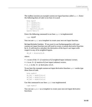
![11 Advanced Topics
Weight Functions
Weight functions calculate a weighted input vector (or matrix) Z given an input
vector (or matrices) P and a weight matrix W.
Once defined you can assign your weight function to any input weight or layer
weight of a network. For example, the following line of code assigns the weight
function yourwf to the weight going to the second layer from the first input of
a network.
net.inputWeights{2,1}.weightFcn = 'yourwf';
Your weight function will then be used whenever you simulate your network.
[Y,Pf,Af] = sim(net,P,Pi,Ai)
To be a valid weight function your function must calculate weight inputs Z from
inputs P and a weight matrix W as follows,
Z = yourwf(W,P)
where:
• W is an S × R weight matrix.
• P is an R × Q matrix of Q input (column) vectors.
• Z is an S × Q matrix of Q weighted input (column) vectors.
Your net input function must also provide information about itself using this
calling format,
info = yourwf(code)
where the correct information is returned for each of the following string codes:
• 'version' - Returns the Neural Network Toolbox version (3.0).
• 'deriv' - Returns the name of the associated derivative function.
The toolbox contains an example custom weight called mywf. Enter the
following lines of code to see how it is used.
help mywf
w = rand(1,5);
p = rand(5,1);
z = mywf(w,p);
mywf('deriv')
11-24](https://image.slidesharecdn.com/nnet-090922002848-phpapp01/85/Neural-Network-Toolbox-MATLAB-348-320.jpg)
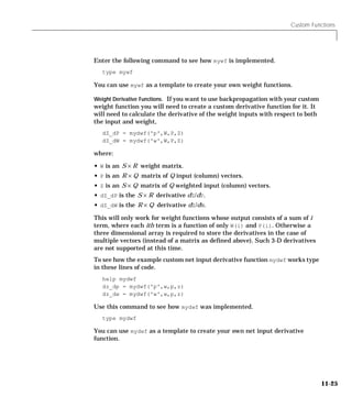
![11 Advanced Topics
initialize the weight and biases it is assigned to whenever you initialize your
network with init.
net = init(net)
To be a valid weight and bias initialization function your function must take a
the number of neurons in a layer S, and a two column matrix PR of R rows
defining the minimum and maximum values of R inputs and return a new
weight matrix W,
W = rands(S,PR)
where:
• S is the number of neurons in the layer.
• PR is an R × 2 matrix defining the minimum and maximum values of R
inputs.
• W is a new S × R weight matrix.
Your function also needs to generate a new bias vector as follows,
b = rands(S)
where:
• S is the number of neurons in the layer.
• b is a new S × 1 bias vector.
To see how an example custom weight and bias initialization function works
type in these lines of code.
help mywbif
W = mywbif(4,[0 1; -2 2])
b = mywbif(4,[1 1])
Use this command to see how mywbif was implemented.
type mywbif
You can use mywbif as a template to create your own weight and bias
initialization function.
11-28](https://image.slidesharecdn.com/nnet-090922002848-phpapp01/85/Neural-Network-Toolbox-MATLAB-352-320.jpg)
![Custom Functions
Learning Functions
You can create three kinds of initialization functions: training, adaption,
performance, and weight/bias learning functions.
Training Functions
One kind of general learning function is a network training function. Training
functions repeatedly apply a set of input vectors to a network, updating the
network each time, until some stopping criteria is met. Stopping criteria can
consists of a maximum number of epochs, a minimum error gradient, an error
goal, etc.
Once defined you can assign your training function to a network.
net.trainFcn = 'yourtf';
Your network initialization function will then be used whenever you train your
network.
[net,tr] = train(NET,P,T,Pi,Ai)
To be a valid training function your function must take and return a network,
[net,tr] = yourtf(net,Pd,Tl,Ai,Q,TS,VV,TV)
where:
• Pd is an N l × N i × TS cell array of tap delayed inputs.
j ij
- Each Pd{i,j,ts} is the R × ( D i Q ) delayed input matrix to the weight
going to the ith layer from the jth input at time step ts. (Pd{i,j,ts} is
an empty matrix [] if the ith layer doesn’t have a weight from the jth
input.)
• Tl is an N l × TS cell array of layer targets.
i
- Each Tl{i,ts} is the S × Q target matrix for the ith layer. (Tl{i,ts} is
an empty matrix if the ith layer doesn’t have a target.)
• Ai is an N l × LD cell array of initial layer delay states.
i
- Each Ai{l,k} is the S × Q delayed ith layer output for time step ts =
k-LD, where ts goes from 0 to LD-1.
• Q is the number of concurrent vectors.
11-29](https://image.slidesharecdn.com/nnet-090922002848-phpapp01/85/Neural-Network-Toolbox-MATLAB-353-320.jpg)
![11 Advanced Topics
Adapt Functions
The other kind of the general learning functions is a network adapt function.
Adapt functions simulate a network, while updating them for each time step of
the input before continuing the simulation to the next input.
Once defined you can assign your training function to a network.
net.adaptFcn = 'youraf';
Your network initialization function will then be used whenever you adapt
your network.
[net,Y,E,Pf,Af] = adapt(NET,P,T,Pi,Ai)
To be a valid training function your function must take and return a network,
[net,Ac,El] = youraf(net,Pd,Tl,Ai,Q,TS)
where:
• Pd is an N l × N i × TS cell array of tap delayed inputs.
j ij
- Each Pd{i,j,ts} is the R × ( D i Q ) delayed input matrix to the weight
going to the ith layer from the jth input at time step ts. (Pd{i,j,ts} is
an empty matrix [] if the ith layer doesn’t have a weight from the jth
input.)
• Tl is an N l × TS cell array of layer targets.
i
- Each Tl{i,ts} is the S × Q target matrix for the ith layer. (Tl{i,ts} is
an empty matrix if the ith layer doesn’t have a target.)
• Ai is an N l × LD cell array of initial layer delay states.
i
- Each Ai{l,k} is the S × Q delayed ith layer output for time step ts =
k-LD, where ts goes from 0 to LD-1.
• Q is the number of concurrent vectors.
• TS is the number of time steps.
11-32](https://image.slidesharecdn.com/nnet-090922002848-phpapp01/85/Neural-Network-Toolbox-MATLAB-356-320.jpg)
![11 Advanced Topics
These functions are not listed in Chapter 13 because they may be altered in the
future. However, you can use these functions if you are willing to take the risk
that you will have to update your functions for future versions of the toolbox.
These two functions are useful for simulating a network, and calculating its
derivatives of performance.
• calca1 - New training record with any number of optional fields.
• calce1 - Clip training record to the final number of epochs.
• calcgrad - Calculate bias and weight performance gradients.
Performance Functions
Performance functions allow a network’s behavior to be graded. This is useful
for many algorithms, such as backpropagation, which operate by adjusting
network weights and biases to improve performance.
Once defined you can assign your training function to a network.
net.performFcn = 'yourpf';
Your network initialization function will then be used whenever you train your
adapt your network.
[net,tr] = train(NET,P,T,Pi,Ai)
[net,Y,E,Pf,Af] = adapt(NET,P,T,Pi,Ai)
To be a valid performance function your function must be called as follows,
perf = yourpf(E,X,PP)
where:
• E is either an S × Q matrix or an N l × TS cell array of layer errors.
i
- Each E{i,ts} is the S × Q target matrix for the ith layer. (Tl(i,ts) is an
empty matrix if the ith layer doesn’t have a target.)
• X is an M × 1 vector of all the network’s weights and biases.
• PP is a structure of network performance parameters.
If E is a cell array you can convert it to a matrix as follows.
E = cell2mat(E);
11-34](https://image.slidesharecdn.com/nnet-090922002848-phpapp01/85/Neural-Network-Toolbox-MATLAB-358-320.jpg)

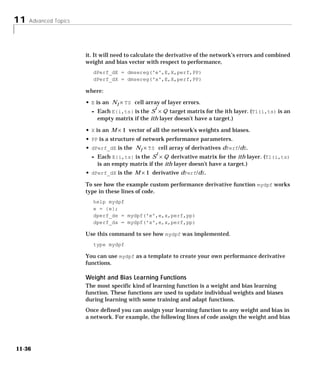
![Custom Functions
learning function yourwblf to the second layer’s bias, and the weight coming
from the first input to the second layer.
net.biases{2}.learnFcn = 'yourwblf';
net.inputWeights{2,1}.learnFcn = 'yourwblf';
Weight and bias initialization functions are only called to update weights and
biases if the network training function (net.trainFcn) is set to either toolbox
function trainwb or trainwb1, or if the network adapt function (net.adaptFcn)
is set to adaptwb. If this is the case, then your function will be used to update
the weight and biases it is assigned to whenever you train or adapt your
network with train or adapt.
[net,tr] = train(NET,P,T,Pi,Ai)
[net,Y,E,Pf,Af] = adapt(NET,P,T,Pi,Ai)
To be a valid weight and bias learning function your function must be callable
as follows,
[dW,LS] = yourwblf(W,P,Z,N,A,T,E,gW,gA,D,LP,LS)
where:
• W is an S × R weight matrix.
• P is an R × Q matrix of Q input (column) vectors.
• Z is an S × Q matrix of Q weighted input (column) vectors.
• N is an S × Q matrix of Q net input (column) vectors.
• A is an S × Q matrix of Q layer output (column) vectors.
• T is an S × Q matrix of Q target (column) vectors.
• E is an S × Q matrix of Q error (column) vectors.
• gW is an S × R gradient of W with respect to performance.
• gA is an S × Q gradient of A with respect to performance.
• D is an S × S matrix of neuron distances.
• LP is a a structure of learning parameters.
• LS is a structure of the learning state which is updated each call. (Use a null
matrix [] the first time.)
• dW is the resulting S × R weight change matrix.
11-37](https://image.slidesharecdn.com/nnet-090922002848-phpapp01/85/Neural-Network-Toolbox-MATLAB-361-320.jpg)
![11 Advanced Topics
Your function will be called as follows to update bias vector.
[db,LS] = yourwblf(b,ones(1,Q),Z,N,A,T,E,gW,gA,D,LP,LS)
where:
• S is the number of neurons in the layer.
• b is a new S × 1 bias vector.
Your learning function must also provide information about itself using this
calling format,
info = yourwblf(code)
where the correct information is returned for each of the following string codes:
• 'version' - Returns the Neural Network Toolbox version (3.0).
• 'deriv' - Returns the name of the associated derivative function.
• 'pdefaults' - Returns a structure of default performance parameters.
To see how an example custom weight and bias initialization function works
type in the example in the following help.
help mywblf
Use this command to see how mywbif was implemented.
type mywblf
You can use mywblf as a template to create your own weight and bias learning
function.
11-38](https://image.slidesharecdn.com/nnet-090922002848-phpapp01/85/Neural-Network-Toolbox-MATLAB-362-320.jpg)
![Custom Functions
Self-Organizing Map Functions
There are two kinds of functions which control how neurons in self-organizing
maps respond. They are topology and distance functions.
Topology Functions
Topology functions calculate the positions of a layer’s neurons given its
dimensions.
Once defined you can assign your topology function to any layer of a network.
For example, the following line of code assigns the topology function yourtopf
to the second layer of a network.
net.layers{2}.topologyFcn = 'yourtopf';
Your topology function will then be used whenever your network is trained or
adapts.
[net,tr] = train(NET,P,T,Pi,Ai)
[net,Y,E,Pf,Af] = adapt(NET,P,T,Pi,Ai)
To be a valid topology function your function must calculate positions pos from
dimensions dim as follows,
pos = yourtopf(dim1,dim2,...,dimN)
where:
• dimi is the number of neurons along the ith dimension of the layer.
• pos is an N × S matrix of S position vectors, where S is the total number of
neurons which is defined by the product dim1*dim1*...*dimN.
The toolbox contains an example custom topology function called mytopf. Enter
the following lines of code to see how it is used.
help mytopf
pos = mytopf(20,20);
plotsom(pos)
11-39](https://image.slidesharecdn.com/nnet-090922002848-phpapp01/85/Neural-Network-Toolbox-MATLAB-363-320.jpg)
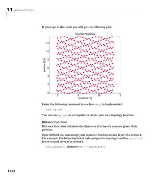
![Custom Functions
Your distance function will then be used whenever your network is trained or
adapts.
[net,tr] = train(NET,P,T,Pi,Ai)
[net,Y,E,Pf,Af] = adapt(NET,P,T,Pi,Ai)
To be a valid distance function your function must calculate distances d from
position pos as follows,
pos = yourtopf(dim1,dim2,...,dimN)
where:
• pos is an N × S matrix of S neuron position vectors.
• d is an S × S matrix of neuron distances.
The toolbox contains an example custom distance function called mydistf.
Enter the following lines of code to see how it is used.
help mydistf
pos = gridtop(4,5);
d = mydistf(pos)
Enter the following command to see how mytf is implemented.
type mydistf
You can use mydistf as a template to create your own distance function.
11-41](https://image.slidesharecdn.com/nnet-090922002848-phpapp01/85/Neural-Network-Toolbox-MATLAB-365-320.jpg)

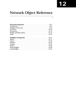

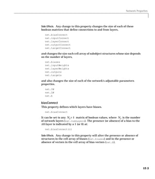
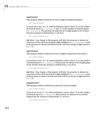

![12 Network Object Reference
It is always set to the maximum delay value associated any of the network’s
input weights.
numInputDelays = 0;
for i=1:net.numLayers
for j=1:net.numInputs
if net.inputConnect(i,j)
numInputDelays = max( ...
[numInputDelays net.inputWeights{i,j}.delays]);
end
end
end
numLayerDelays (read-only)
This property indicates the number of time steps of past layer outputs that
must be supplied to simulate the network.
net.numLayerDelays
It is always set to the maximum delay value associated any of the network’s
layer weights.
numLayerDelays = 0;
for i=1:net.numLayers
for j=1:net.numLayers
if net.layerConnect(i,j)
numLayerDelays = max( ...
[numLayerDelays net.layerWeights{i,j}.delays]);
end
end
end
Subobject Structures
These properties consist of cell arrays of structures which define each of the
network’s inputs, layers, outputs, targets, biases, and weights.
The properties for each kind of subobject are described in the “Subobject
Properties” section which follows this “Network Properties” section.
12-6](https://image.slidesharecdn.com/nnet-090922002848-phpapp01/85/Neural-Network-Toolbox-MATLAB-372-320.jpg)
![Network Properties
inputs
This property holds structures of properties for each of the network’s inputs.
net.inputs
It is always an N i × 1 cell array of input structures, where N i is the number
of network inputs (net.numInputs).
The structure defining the properties of the ith network input is located at:
net.inputs{i}
Input Properties. See “Inputs” in the “Subobject Properties” section for
descriptions of input properties.
layers
This property holds structures of properties for each of the network’s layers.
net.layers
It is always an N l × 1 cell array of input structures, where N l is the number
of network layers (net.numLayers).
The structure defining the properties of the ith layer is located at:
net.layers{i}
Layer Properties. See “Layers” in the “Subobject Properties” section for
descriptions of layer properties.
outputs
This property holds structures of properties for each of the network’s outputs.
net.outputs
It is always an N l × 1 cell array, where N l is the number of network layers
(net.numLayers).
The structure defining the properties of the output from the ith layer (or a null
matrix []) is located at:
net.outputs{i}
12-7](https://image.slidesharecdn.com/nnet-090922002848-phpapp01/85/Neural-Network-Toolbox-MATLAB-373-320.jpg)
![12 Network Object Reference
if the corresponding output connection is 1 (or 0).
net.outputConnect(i)
Output Properties. See “Outputs” in the “Subobject Properties” section for
descriptions of output properties.
targets
This property holds structures of properties for each of the network’s targets.
net.targets
It is always an N l × 1 cell array, where N l is the number of network layers
(net.numLayers).
The structure defining the properties of the target associated with the ith layer
(or a null matrix []) is located at:
net.targets{i}
if the corresponding target connection is 1 (or 0).
net.targetConnect(i)
Target Properties. See “Targets” in the “Subobject Properties” section for
descriptions of target properties.
biases
This property holds structures of properties for each of the network’s biases.
net.biases
It is always an N l × 1 cell array, where N l is the number of network layers
(net.numLayers).
The structure defining the properties of the bias associated with the ith layer
(or a null matrix []) is located at:
net.biases{i}
if the corresponding bias connection is 1 (or 0).
net.biasConnect(i)
12-8](https://image.slidesharecdn.com/nnet-090922002848-phpapp01/85/Neural-Network-Toolbox-MATLAB-374-320.jpg)
![Network Properties
Bias Properties. See “Biases” in the “Subobject Properties” section for
descriptions of bias properties.
inputWeights
This property holds structures of properties for each of the network’s input
weights.
net.inputWeights
It is always an N l × N i cell array, where N l is the number of network layers
(net.numLayers) and N i is the number of network inputs (net.numInputs).
The structure defining the properties of the weight going to the ith layer from
the jth input (or a null matrix []) is located at:
net.inputWeights{i,j}
if the corresponding input connection is 1 (or 0).
net.inputConnect(i,j)
Input Weight Properties. See “Input Weights” in the “Subobject Properties” section
for descriptions of input weight properties.
layerWeights
This property holds structures of properties for each of the network’s layer
weights.
net.layerWeights
It is always an N l × N l cell array, where N l is the number of network layers
(net.numLayers).
The structure defining the properties of the weight going to the ith layer from
the jth layer (or a null matrix []) is located at:
net.layerWeights{i,j}
if the corresponding layer connection is 1 (or 0).
net.layerConnect(i,j)
Layer Weight Properties. See “LayerWeights” in the “Subobject Properties” section
for descriptions of layer weight properties.
12-9](https://image.slidesharecdn.com/nnet-090922002848-phpapp01/85/Neural-Network-Toolbox-MATLAB-375-320.jpg)
![12 Network Object Reference
Functions
These properties define the algorithms to use when a network is to adapt, is to
be initialized, is to have its performance measured, or is to be trained.
adaptFcn
This property defines the function to be used when the network adapts.
net.adaptFcn
It can be set to the name of any network adapt function, including this toolbox
function:
adaptwb - By-weight-and-bias network adaption function.
The network adapt function is used to perform adaption whenever adapt is
called.
[net,Y,E,Pf,Af] = adapt(NET,P,T,Pi,Ai)
Custom Functions. See Chapter 11, “Advanced Topics” for information on creating
custom adapt functions.
Side Effects. Whenever this property is altered the network’s adaption
parameters (net.adaptParam) are set to contain the parameters and default
values of the new function.
initFcn
This property defines the function used to initialize the network’s weight
matrices and bias vectors.
net.initFcn
It can be set to the name of any network initialization function, including this
toolbox function.
initlay - Layer-by-layer network initialization function.
The initialization function is used to initialize the network whenever init is
called.
net = init(net)
12-10](https://image.slidesharecdn.com/nnet-090922002848-phpapp01/85/Neural-Network-Toolbox-MATLAB-376-320.jpg)
![Network Properties
Custom Functions. See Chapter 11, “Advanced Topics” for information on creating
custom initialization functions.
Side Effects. Whenever this property is altered the network’s initialization
parameters (net.initParam) are set to contain the parameters and default
values of the new function.
performFcn
This property defines the function used to measure the network’s performance.
net.performFcn
It can be set to the name of any performance function, including these toolbox
functions:
Performance Functions
mae Mean absolute error performance function.
mse Mean squared error performance function.
msereg Mean squared error w/reg performance function.
sse Sum squared error performance function.
The performance function is used to calculate network performance during
training whenever train is called.
[net,tr] = train(NET,P,T,Pi,Ai)
Custom functions. See Chapter 11, “Advanced Topics” for information on creating
custom performance functions.
Side Effects. Whenever this property is altered the network’s performance
parameters (net.performParam) are set to contain the parameters and default
values of the new function.
trainFcn
This property defines the function used to train the network.
net.trainFcn
12-11](https://image.slidesharecdn.com/nnet-090922002848-phpapp01/85/Neural-Network-Toolbox-MATLAB-377-320.jpg)
![12 Network Object Reference
It can be set to the name of any training function, including these toolbox
functions:
Training Functions
trainbfg BFGS quasi-Newton backpropagation.
trainbr Bayesian regularization.
traincgb Powell-Beale conjugate gradient backpropagation.
traincgf Fletcher-Powell conjugate gradient backpropagation.
traincgp Polak-Ribiere conjugate gradient backpropagation.
traingd Gradient descent backpropagation.
traingda Gradient descent w/adaptive lr backpropagation.
traingdm Gradient descent w/momentum backpropagation.
traingdx Gradient descent w/momentum & adaptive lr backprop.
trainlm Levenberg-Marquardt backpropagation.
trainoss One step secant backpropagation.
trainrp Resilient backpropagation (Rprop)
trainscg Scaled conjugate gradient backpropagation.
trainwb By-weight-and-bias network training function.
trainwb1 By-weight-&-bias 1-vector-at-a-time training function.
The training function is used to train the network whenever train is called.
[net,tr] = train(NET,P,T,Pi,Ai)
Custom Functions. See Chapter 11, “Advanced Topics” for information on creating
custom training functions.
Side Effects. Whenever this property is altered the network’s training
parameters (net.trainParam) are set to contain the parameters and default
values of the new function.
12-12](https://image.slidesharecdn.com/nnet-090922002848-phpapp01/85/Neural-Network-Toolbox-MATLAB-378-320.jpg)
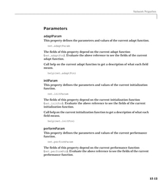
![12 Network Object Reference
Call help on the current performance function to get a description of what each
field means.
help(net.performFcn)
trainParam
This property defines the parameters and values of the current training
function.
net.trainParam
The fields of this property depend on the current training function
(net.trainFcn). Evaluate the above reference to see the fields of the current
training function.
Call help on the current training function to get a description of what each field
means.
help(net.trainFcn)
Weight and Bias Values
These properties define the network’s adjustable parameters: its weight
matrices and bias vectors.
IW
This property defines the weight matrices of weights going to layers from
network inputs.
net.IW
It is always an N l × N i cell array, where N l is the number of network layers
(net.numLayers) and N i is the number of network inputs (net.numInputs).
The weight matrix for the weight going to the ith layer from the jth input (or a
null matrix []) is located at:
net.IW{i,j}
if the corresponding input connection is 1 (or 0).
net.inputConnect(i,j)
12-14](https://image.slidesharecdn.com/nnet-090922002848-phpapp01/85/Neural-Network-Toolbox-MATLAB-380-320.jpg)
![Network Properties
The weight matrix will have as many rows as the size of the layer it goes to
(net.layers{i}.size). It will have as many columns as the product of the
input size with the number of delays associated with the weight.
net.inputs{j}.size * length(net.inputWeights{i,j}.delays)
These dimensions can also be obtained from the input weight properties.
net.inputWeights{i,j}.size
LW
This property defines the weight matrices of weights going to layers from other
layers.
net.LW
It is always an N l × N l cell array, where N l is the number of network layers
(net.numLayers).
The weight matrix for the weight going to the ith layer from the jth layer (or a
null matrix []) is located at:
net.LW{i,j}
if the corresponding layer connection is 1 (or 0).
net.layerConnect(i,j)
The weight matrix will have as many rows as the size of the layer it goes to
(net.layers{i}.size). It will have as many columns as the product of the size
of the layer it comes from with the number of delays associated with the
weight.
net.layers{j}.size * length(net.layerWeights{i,j}.delays)
These dimensions can also be obtained from the layer weight properties.
net.layerWeights{i,j}.size
12-15](https://image.slidesharecdn.com/nnet-090922002848-phpapp01/85/Neural-Network-Toolbox-MATLAB-381-320.jpg)
![12 Network Object Reference
b
This property defines the bias vectors for each layer with a bias.
net.b
It is always an N l × 1 cell array, where N l is the number of network layers
(net.numLayers).
The bias vector for the ith layer (or a null matrix []) is located at:
net.b{i}
if the corresponding bias connection is 1 (or 0).
net.biasConnect(i)
The number of elements in the bias vector is always equal to the size of the
layer it is associated with (net.layers{i}.size).
This dimension can also be obtained from the bias properties.
net.biases{i}.size
Other
The only other property is a user data property.
userdata
This property provides a place for users to add custom information to a network
object.
net.userdata
Only one field is predefined. It contains a secret message to all Neural Network
Toolbox users.
net.userdata.note
Please keep this information confidential.
12-16](https://image.slidesharecdn.com/nnet-090922002848-phpapp01/85/Neural-Network-Toolbox-MATLAB-382-320.jpg)

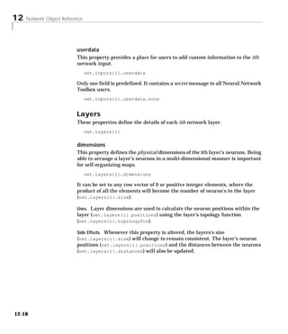
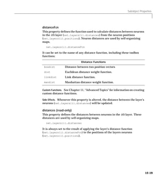
![12 Network Object Reference
initFcn
This property defines the initialization function used to initialize the ith layer,
if the network initialization function (net.initFcn) is initlay.
net.layers{i}.initFcn
It can be set to the name of any layer initialization function, including these
toolbox functions:
Layer Initialization Functions
initnw Nguyen-Widrow layer initialization function.
initwb By-weight-and-bias layer initialization function
If the network initialization is set to initlay, then the function indicated by
this property will be used to initialize the layer’s weights and biases when init
is called.
net = init(net)
Custom Functions. See Chapter 11, “Advanced Topics” for information on creating
custom initialization functions.
netInputFcn
This property defines the net input function use to calculate the ith layer’s net
input, given the layer’s weighted inputs and bias.
net.layers{i}.netInputFcn
It can be set to the name of any net input function, including these toolbox
functions:
Net Input Functions
netprod Product net input function.
netsum Sum net input function.
The net input function is used to simulate the network when sim is called.
[Y,Pf,Af] = sim(net,P,Pi,Ai)
12-20](https://image.slidesharecdn.com/nnet-090922002848-phpapp01/85/Neural-Network-Toolbox-MATLAB-386-320.jpg)
![Subobject Properties
Custom Functions. See Chapter 11, “Advanced Topics” for information on creating
custom net input functions.
positions (read-only)
This property defines the positions of neurons in the ith layer. These positions
are used by self-organizing maps.
net.layers{i}.positions
It is always set to the result of applying the layer’s topology function
(net.layers{i}.topologyFcn) to the positions of the layer’s dimensions
(net.layers{i}.dimensions).
Plotting. Use plotsom to plot the positions of a layer’s neurons.
For instance, if the first layer neurons of a network are arranged with
dimensions (net.layers{1}.dimensions) of [4 5] and the topology function
(net.layers{1}.topologyFcn) is hextop, the neuron’s positions can be plotted
as shown below.
plotsom(net.layers{1}.positions)
Neuron Positions
3
2.5
position(2,i)
2
1.5
1
0.5
0
0 1 2 3
position(1,i)
12-21](https://image.slidesharecdn.com/nnet-090922002848-phpapp01/85/Neural-Network-Toolbox-MATLAB-387-320.jpg)
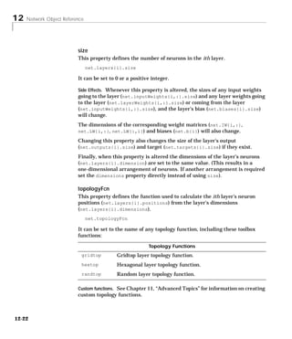
![Subobject Properties
Side Effects. Whenever this property is altered, the positions of the layer’s
neurons (net.layers{i}.positions) will be updated.
Plotting. Use plotsom to plot the positions of a layer’s neurons.
For instance, if the first layer neurons of a network are arranged with
dimensions (net.layers{1}.dimensions) of [8 10] and the topology function
(net.layers{1}.topologyFcn) is randtop, the neuron’s positions will be
arranged something like those shown in the plot below.
plotsom(net.layers{1}.positions)
Neuron Positions
6
5
4
position(2,i)
3
2
1
0
0 1 2 3 4 5 6
position(1,i)
transferFcn
This function defines the transfer function use to calculate the ith layer’s
output, given the layer’s net input.
net.layers{i}.transferFcn
12-23](https://image.slidesharecdn.com/nnet-090922002848-phpapp01/85/Neural-Network-Toolbox-MATLAB-389-320.jpg)
![12 Network Object Reference
It can be set to the name of any transfer function, including these toolbox
functions:
Transfer Functions
compet Competitive transfer function.
hardlim Hard limit transfer function.
hardlims Symmetric hard limit transfer function.
logsig Log sigmoid transfer function.
poslin Positive linear transfer function.
purelin Hard limit transfer function.
radbas Radial basis transfer function.
satlin Saturating linear transfer function.
satlins Symmetric saturating linear transfer function.
softmax Soft max transfer function.
tansig Hyperbolic tangent sigmoid transfer function.
tribas Triangular basis transfer function
The transfer function is used to simulate the network when sim is called.
[Y,Pf,Af] = sim(net,P,Pi,Ai)
Custom functions. See Chapter 11, “Advanced Topics” for information on creating
custom transfer functions.
userdata
This property provides a place for users to add custom information to the ith
network layer.
net.layers{i}.userdata
Only one field is predefined. It contains a secret message to all Neural Network
Toolbox users.
net.layers{i}.userdata.note
12-24](https://image.slidesharecdn.com/nnet-090922002848-phpapp01/85/Neural-Network-Toolbox-MATLAB-390-320.jpg)
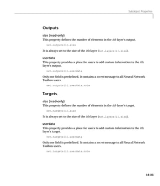
![12 Network Object Reference
Biases
initFcn
This property defines the function used to initialize the ith layer’s bias vector,
if the network initialization function is initlay, and the ith layer’s
initialization function is initwb.
net.biases{i}.initFcn
This function can be set to the name of any bias initialization function,
including the toolbox functions:
Bias Initialization Functions
initcon Conscience bias initialization function.
initzero Zero weight/bias initialization function.
rands Symmetric random weight/bias initialization function.
This function will be used to calculate an initial bias vector for the ith layer
(net.b{i}) when init is called, if the network initialization function
(net.initFcn) is initlay, and the ith layer’s initialization function
(net.layers{i}.initFcn) is initwb.
net = init(net)
Custom functions. See Chapter 11, “Advanced Topics” for information on creating
custom initialization functions.
learn
This property defines whether the ith bias vector is to be altered during
training and adaption.
net.biases{i}.learn
It can be set to 0 or 1.
It enables or disables the bias’ learning during calls to either adapt or train.
[net,Y,E,Pf,Af] = adapt(NET,P,T,Pi,Ai)
[net,tr] = train(NET,P,T,Pi,Ai)
12-26](https://image.slidesharecdn.com/nnet-090922002848-phpapp01/85/Neural-Network-Toolbox-MATLAB-392-320.jpg)
![Subobject Properties
learnFcn
This property defines the function used to update the ith layer’s bias vector
during training, if the network training function is trainwb or trainwb1, or
during adaption, if the network adapt function is adaptwb.
net.biases{i}.learnFcn
It can be set to the name of any bias learning function, including these toolbox
functions:
Learning Functions
learncon Conscience bias learning function.
learngd Gradient descent weight/bias learning function
learngdm Grad. descent w/momentum weight/bias learning function
learnp Perceptron weight/bias learning function.
learnpn Normalized perceptron weight/bias learning function.
learnwh Widrow-Hoff weight/bias learning rule
The learning function will update the ith bias vector (net.b{i}) during calls to
train, if the network training function (net.trainFcn) is trainwb or trainwb1,
or during calls to adapt, if the network adapt function (net.adaptFcn) is
adaptwb.
[net,Y,E,Pf,Af] = adapt(NET,P,T,Pi,Ai)
[net,tr] = train(NET,P,T,Pi,Ai)
Custom functions. See Chapter 11, “Advanced Topics” for information on creating
custom learning functions.
Side Effects. Whenever this property is altered the biases’s learning parameters
(net.biases{i}.learnParam) are set to contain the fields and default values of
the new function.
learnParam
This property defines the learning parameters and values for the current
learning function of the ith layer’s bias.
net.biases{i}.learnParam
12-27](https://image.slidesharecdn.com/nnet-090922002848-phpapp01/85/Neural-Network-Toolbox-MATLAB-393-320.jpg)
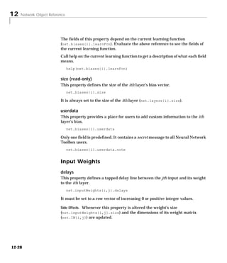
![Subobject Properties
initFcn
This property defines the function used to initialize the weight matrix going to
the ith layer from the jth input, if the network initialization function is
initlay, and the ith layer’s initialization function is initwb.
net.inputWeights{i,j}.initFcn
This function can be set to the name of any weight initialization function,
including these toolbox functions:
Weight Initialization Functions
initzero Zero weight/bias initialization function.
midpoint Midpoint weight initialization function.
randnc Normalized column weight initialization function.
randnr Normalized row weight initialization function.
rands Symmetric random weight/bias initialization function.
This function will be used to calculate an initial weight matrix for the weight
going to the ith layer from the jth input (net.IW{i,j}) when init is called, if
the network initialization function (net.initFcn) is initlay, and the ith
layer’s initialization function (net.layers{i}.initFcn) is initwb.
net = init(net)
Custom Functions. See Chapter 11, “Advanced Topics” for information on creating
custom initialization functions.
learn
This property defines whether the weight matrix to the ith layer from the jth
input is to be altered during training and adaption.
net.inputWeights{i,j}.learn
It can be set to 0 or 1.
It enables or disables the weights learning during calls to either adapt or
train.
[net,Y,E,Pf,Af] = adapt(NET,P,T,Pi,Ai)
[net,tr] = train(NET,P,T,Pi,Ai)
12-29](https://image.slidesharecdn.com/nnet-090922002848-phpapp01/85/Neural-Network-Toolbox-MATLAB-395-320.jpg)
![12 Network Object Reference
learnFcn
This property defines the function used to update the weight matrix going to
the ith layer from the jth input during training, if the network training function
is trainwb or trainwb1, or during adaption, if the network adapt function is
adaptwb.
net.inputWeights{i,j}.learnFcn
It can be set to the name of any weight learning function, including these
toolbox functions:
Weight Learning Functions
learngd Gradient descent weight/bias learning function
learngdm Grad. descent w/momentum weight/bias learning function
learnh Hebb weight learning function.
learnhd Hebb with decay weight learning function.
learnis Instar weight learning function.
learnk Kohonen weight learning function.
learnlv1 LVQ1 weight learning function.
learnlv2 LVQ2 weight learning function.
learnos Outstar weight learning function.
learnp Perceptron weight/bias learning function.
learnpn Normalized perceptron weight/bias learning function.
learnsom Self-organizing map weight learning function.
learnwh Widrow-Hoff weight/bias learning rule
The learning function will update the weight matrix of the ith layer form the
jth input (net.IW{i,j}) during calls to train, if the network training function
(net.trainFcn) is trainwb or trainwb1, or during calls to adapt, if the network
adapt function (net.adaptFcn) is adaptwb.
[net,Y,E,Pf,Af] = adapt(NET,P,T,Pi,Ai)
[net,tr] = train(NET,P,T,Pi,Ai)
12-30](https://image.slidesharecdn.com/nnet-090922002848-phpapp01/85/Neural-Network-Toolbox-MATLAB-396-320.jpg)
![12 Network Object Reference
weightFcn
This property defines the function used to apply the ith layer’s weight from the
jth input to that input.
net.inputWeights{i,j}.weightFcn
It can be set to the name of any weight function, including these toolbox
functions:
Weight Functions
dist Conscience bias initialization function.
dotprod Zero weight/bias initialization function.
mandist Manhattan distance weight function.
negdist Normalized column weight initialization function.
normprod Normalized row weight initialization function.
The weight function is used when sim is called to simulate the network.
[Y,Pf,Af] = sim(net,P,Pi,Ai)
Custom functions. See Chapter 11, “Advanced Topics” for information on creating
custom weight functions.
LayerWeights
delays
This property defines a tapped delay line between the jth layer and its weight
to the ith layer.
net.layerWeights{i,j}.delays
It must be set to a row vector of increasing 0 or positive integer values.
initFcn
This property defines the function used to initialize the weight matrix going to
the ith layer from the jth layer, if the network initialization function is
initlay, and the ith layer’s initialization function is initwb.
net.layerWeights{i,j}.initFcn
12-32](https://image.slidesharecdn.com/nnet-090922002848-phpapp01/85/Neural-Network-Toolbox-MATLAB-398-320.jpg)
![Subobject Properties
This function can be set to the name of any weight initialization function,
including the toolbox functions:
Weight and Bias Initialization Functions
initzero Zero weight/bias initialization function.
midpoint Midpoint weight initialization function.
randnc Normalized column weight initialization function.
randnr Normalized row weight initialization function.
rands Symmetric random weight/bias initialization function.
This function will be used to calculate an initial weight matrix for the weight
going to the ith layer from the jth layer (net.LW{i,j}) when init is called, if
the network initialization function (net.initFcn) is initlay, and the ith
layer’s initialization function (net.layers{i}.initFcn) is initwb.
net = init(net)
Custom Functions. See Chapter 11, “Advanced Topics” for information on creating
custom initialization functions.
learn
This property defines whether the weight matrix to the ith layer from the jth
layer is to be altered during training and adaption.
net.layerWeights{i,j}.learn
It can be set to 0 or 1.
It enables or disables the weights learning during calls to either adapt or
train.
[net,Y,E,Pf,Af] = adapt(NET,P,T,Pi,Ai)
[net,tr] = train(NET,P,T,Pi,Ai)
learnFcn
This property defines the function used to update the weight matrix going to
the ith layer from the jth layer during training, if the network training function
12-33](https://image.slidesharecdn.com/nnet-090922002848-phpapp01/85/Neural-Network-Toolbox-MATLAB-399-320.jpg)
![12 Network Object Reference
is trainwb or trainwb1, or during adaption, if the network adapt function is
adaptwb.
net.layerWeights{i,j}.learnFcn
It can be set to the name of any weight learning function, including these
toolbox functions:
Learning Functions
learngd Gradient descent weight/bias learning function
learngdm Grad. descent w/momentum weight/bias learning function
learnh Hebb weight learning function.
learnhd Hebb with decay weight learning function.
learnis Instar weight learning function.
learnk Kohonen weight learning function.
learnlv1 LVQ1 weight learning function.
learnlv2 LVQ2 weight learning function.
learnos Outstar weight learning function.
learnp Perceptron weight/bias learning function.
learnpn Normalized perceptron weight/bias learning function.
learnsom Self-organizing map weight learning function.
learnwh Widrow-Hoff weight/bias learning rule
The learning function will update the weight matrix of the ith layer form the
jth layer (net.LW{i,j}) during calls to train, if the network training function
(net.trainFcn) is trainwb or trainwb1, or during calls to adapt, if the network
adapt function (net.adaptFcn) is adaptwb.
[net,Y,E,Pf,Af] = adapt(NET,P,T,Pi,Ai)
[net,tr] = train(NET,P,T,Pi,Ai)
Custom Functions. See Chapter 11, “Advanced Topics” for information on creating
custom learning functions.
12-34](https://image.slidesharecdn.com/nnet-090922002848-phpapp01/85/Neural-Network-Toolbox-MATLAB-400-320.jpg)
![12 Network Object Reference
weightFcn
This property defines the function used to apply the ith layer’s weight from the
jth layer to that layer’s output.
net.layerWeights{i,j}.weightFcn
It can be set to the name of any weight function, including these toolbox
functions:
Weight Functions
dist Euclidean distance weight function.
dotprod Dot product weight function.
mandist Manhattan distance weight function.
negdist Dot product weight function.
normprod Normalized dot product weight function.
The weight function is used when sim is called to simulate the network.
[Y,Pf,Af] = sim(net,P,Pi,Ai)
Custom Functions. See Chapter 11, “Advanced Topics” for information on creating
custom weight functions.
12-36](https://image.slidesharecdn.com/nnet-090922002848-phpapp01/85/Neural-Network-Toolbox-MATLAB-402-320.jpg)
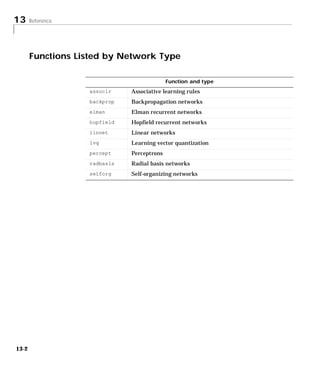
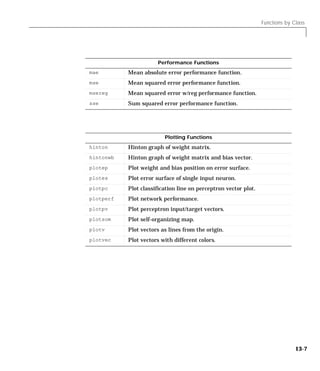
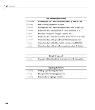
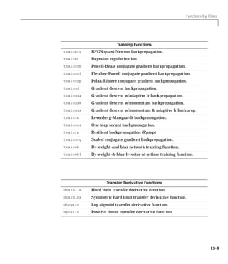

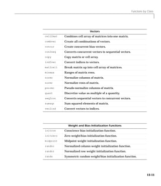

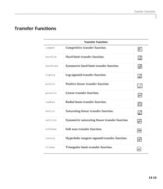
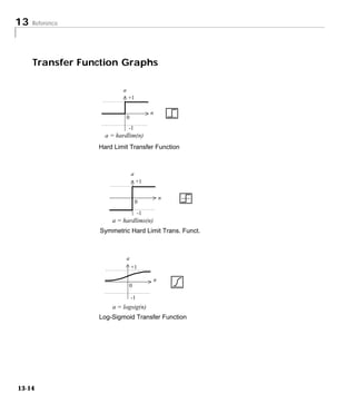
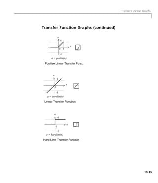
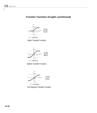
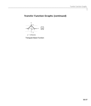

![adapt
Purpose Allow a neural network to adapt
adapt
Syntax [net,Y,E,Pf,Af] = adapt(net,P,T,Pi,Ai)
To Get Help Type help network/adapt
Description [net,Y,E,Pf,Af] = adapt(net,P,T,Pi,Ai) takes,
net - Network.
P - Network inputs.
T - Network targets, default = zeros.
Pi - Initial input delay conditions, default = zeros.
Ai - Initial layer delay conditions, default = zeros.
and returns the following after applying the adapt function net.adaptFcn with
the adaption parameters net.adaptParam:
net - Updated network.
Y - Network outputs.
E - Network errors.
Pf - Final input delay conditions.
Af - Final layer delay conditions.
Note that T is optional and only needs to be used for networks that require
targets. Pi and Pf are also optional and only needs to be used for networks that
have input or layer delays.
adapt's signal arguments can have two formats: cell array or matrix.
13-19](https://image.slidesharecdn.com/nnet-090922002848-phpapp01/85/Neural-Network-Toolbox-MATLAB-421-320.jpg)
![adapt
Each matrix argument is found by storing the elements of the corresponding
cell array argument in a single matrix:
P - (sum of Ri) x Q matrix
T - (sum of Vi) x Q matrix
Pi - (sum of Ri) x (ID*Q) matrix.
Ai - (sum of Si) x (LD*Q) matrix.
Y - (sum of Ui) x Q matrix.
Pf - (sum of Ri) x (ID*Q) matrix.
Af - (sum of Si) x (LD*Q) matrix.
Examples Here two sequences of 12 steps (where T1 is known to depend on P1) are used
to define the operation of a filter.
p1 = {-1 0 1 0 1 1 -1 0 -1 1 0 1};
t1 = {-1 -1 1 1 1 2 0 -1 -1 0 1 1};
Here newlin is used to create a layer with an input range of [-1 1]), one
neuron, input delays of 0 and 1, and a learning rate of 0.5. The linear layer is
then simulated.
net = newlin([-1 1],1,[0 1],0.5);
Here the network adapts for one pass through the sequence.
The network's mean squared error is displayed. (Since this is the first call of
adapt the default Pi is used.)
[net,y,e,pf] = adapt(net,p1,t1);
mse(e)
Note the errors are quite large. Here the network adapts to another 12 time
steps (using the previous Pf as the new initial delay conditions.)
p2 = {1 -1 -1 1 1 -1 0 0 0 1 -1 -1};
t2 = {2 0 -2 0 2 0 -1 0 0 1 0 -1};
[net,y,e,pf] = adapt(net,p2,t2,pf);
mse(e)
13-21](https://image.slidesharecdn.com/nnet-090922002848-phpapp01/85/Neural-Network-Toolbox-MATLAB-423-320.jpg)
![adapt
Here the network adapts for 100 passes through the entire sequence.
p3 = [p1 p2];
t3 = [t1 t2];
net.adaptParam.passes = 100;
[net,y,e] = adapt(net,p3,t3);
mse(e)
The error after 100 passes through the sequence is very small. The network has
adapted to the relationship between the input and target signals.
Algorithm adapt calls the function indicated by net.adaptFcn, using the adaption
parameter values indicated by net.adaptParam.
Given an input sequence with TS steps the network is updated as follows. Each
step in the sequence of inputs is presented to the network one at a time. The
network's weight and bias values are updated after each step, before the next
step in the sequence is presented. Thus the network is updated TS times.
See Also sim, init, train
13-22](https://image.slidesharecdn.com/nnet-090922002848-phpapp01/85/Neural-Network-Toolbox-MATLAB-424-320.jpg)
![adaptwb
Purpose By-weight-and-bias network adaption function
adaptwb
Syntax [net,Ac,El] = adaptwb(net,Pd,Tl,Ai,Q,TS)
info = adaptwb(code)
Description adaptwb is a network function which updates each weight and bias according
to its learning function.
adaptwb takes these inputs,
net - Neural network.
Pd - Delayed inputs.
Tl - Layer targets.
Ai - Initial input conditions.
Q - Batch size.
TS - Time steps.
After training the network with its weight and bias the learning functions
returns,
net - Updated network.
Ac - Collective layer outputs.
El - Layer errors.
Adaption occurs according to the adaptwb's training parameter, shown here
with its default value:
net.adaptparam.passes 1 Number of passes through sequence
Dimensions for these variables are:
Pd - No x Ni x TS cell array, each element P{i,j,ts} is a Zij x Q matrix.
Tl - Nl x TS cell array, each element P{i,ts} is a Vi x Q matrix or [].
Ai - Nl x LD cell array, each element Ai{i,k} is an Si x Q matrix.
Ac - Nl x (LD+TS) cell array, each element Ac{i,k} is an Si x Q matrix.
El - Nl x TS cell array, each element El{i,k} is an Si x Q matrix or [].
13-23](https://image.slidesharecdn.com/nnet-090922002848-phpapp01/85/Neural-Network-Toolbox-MATLAB-425-320.jpg)
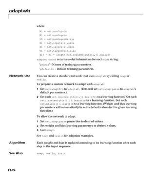
![cell2mat
Purpose Combines a cell array of matrices into one matrix
cell2mat
Syntax m = cell2mat(c)
Description m = cell2mat(C)
C - Cell array of matrices: {M11 M12... ; M21 M22... ; ...}
returns
M - Single matrix: [M11 M12 ...; M21 M22... ; ...]
Examples Examples
c = {[1 2] [3]; [4 5; 6 7] [8; 9]};
m = cell2mat(c)
See Also mat2cell
13-26](https://image.slidesharecdn.com/nnet-090922002848-phpapp01/85/Neural-Network-Toolbox-MATLAB-428-320.jpg)
![combvec
Purpose Create all combinations of vectors
combvec
Syntax combvec(a1,a2)
Description combvec(A1,A2) takes two inputs,
A1 - Matrix of N1 (column) vectors.
A2 - Matrix of N2 (column) vectors.
and returns a matrix of N1*N2 column vectors, where the columns consist of all
possibilities of A2 vectors, appended to A1 vectors.
Examples a1 = [1 2 3; 4 5 6];
a2 = [7 8; 9 10];
a3 = combvec(a1,a2)
13-27](https://image.slidesharecdn.com/nnet-090922002848-phpapp01/85/Neural-Network-Toolbox-MATLAB-429-320.jpg)
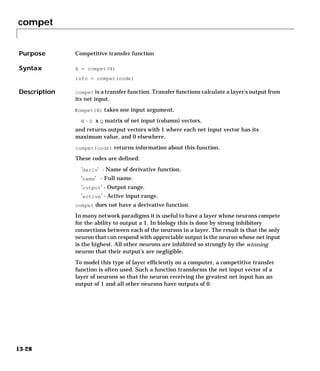
![compet
Examples Here we define a net input vector N, calculate the output, and plot both with
bar graphs.
n = [0; 1; -0.5; 0.5];
a = compet(n);
subplot(2,1,1), bar(n), ylabel('n')
subplot(2,1,2), bar(a), ylabel('a')
Network Use You can create a standard network that uses compet by calling newc or newpnn.
To change a network so a layer uses compet, set
net.layers{i,j}.transferFcn to 'compet'.
In either case, call sim to simulate the network with compet.
See newc or newpnn for simulation examples.
See Also sim, softmax
13-29](https://image.slidesharecdn.com/nnet-090922002848-phpapp01/85/Neural-Network-Toolbox-MATLAB-431-320.jpg)
![con2seq
Purpose Convert concurrent vectors to sequential vectors
con2seq
Syntax s = con2seq(b)
Description The neural network toolbox arranges concurrent vectors with a matrix, and
sequential vectors with a cell array (where the second index is the time step).
con2seq and seq2con allow concurrent vectors to be converted to sequential
vectors, and back again.
con2seq(b)takes one input,
b - R x TS matrix.
and returns one output,
S - 1 x TS cell array of R x 1 vectors.
con2seq(b,TS) can also convert multiple batches,
b - N x 1 cell array of matrices with M*TS columns.
TS - Time steps.
and will return,
S - N x TS cell array of matrices with M columns.
Examples Here a batch of three values is converted to a sequence.
p1 = [1 4 2]
p2 = con2seq(p1)
Here two batches of vectors are converted to two sequences with two time steps.
p1 = {[1 3 4 5; 1 1 7 4]; [7 3 4 4; 6 9 4 1]}
p2 = con2seq(p1,2)
See Also seq2con, concur
13-30](https://image.slidesharecdn.com/nnet-090922002848-phpapp01/85/Neural-Network-Toolbox-MATLAB-432-320.jpg)
![concur
Purpose Create concurrent bias vectors
concur
Syntax concur(b,q)
Description concur(B,Q)
B - S x 1 bias vector (or Nl x 1 cell array of vectors).
Q - Concurrent size.
Returns an S x B matrix of copies of B (or Nl x 1 cell array of matrices).
Examples Here concur creates three copies of a bias vector.
b = [1; 3; 2; -1];
concur(b,3)
Network Use To calculate a layer's net input, the layer's weighted inputs must be combined
with its biases. The following expression calculates the net input for a layer
with the netsum net input function, two input weights, and a bias:
n = netsum(z1,z2,b)
The above expression works if Z1, Z2, and B are all S x 1 vectors. However, if
the network is being simulated by sim (or adapt or train) in response to Q
concurrent vectors, then Z1 and Z2 will be S x Q matrices. Before B can be
combined with Z1 and Z2 we must make Q copies of it.
n = netsum(z1,z2,concur(b,q))
See Also netsum, netprod, sim, seq2con, con2seq
13-31](https://image.slidesharecdn.com/nnet-090922002848-phpapp01/85/Neural-Network-Toolbox-MATLAB-433-320.jpg)
![ddotprod
Purpose Dot product weight derivative function
ddotprod
Syntax dZ_dP = ddotprod('p',W,P,Z)
dZ_dW = ddotprod('w',W,P,Z)
Description ddotprod is a weight derivative function.
ddotprod('p',W,P,Z) takes three arguments,
W - S x R weight matrix.
P - R x Q Inputs.
Z - S x Q weighted input.
and returns the S x R derivative dZ/dP.
ddotprod('w',W,P,Z) returns the R x Q derivative dZ/dW.
Examples Here we define a weight W and input P for an input with 3 elements and a layer
with 2 neurons.
W = [0 -1 0.2; -1.1 1 0];
P = [0.1; 0.6; -0.2];
Here we calculate the weighted input with dotprod, then calculate each
derivative with ddotprod.
Z = dotprod(W,P)
dZ_dP = ddotprod('p',W,P,Z)
dZ_dW = ddotprod('w',W,P,Z)
Algorithm The derivative of a product of two elements with respect to one element is the
other element.
dZ/dP = W
dZ/dW = P
See Also dotprod
13-32](https://image.slidesharecdn.com/nnet-090922002848-phpapp01/85/Neural-Network-Toolbox-MATLAB-434-320.jpg)
![dhardlim
Purpose Derivative of hard limit transfer function
dhardlim
Syntax dA_dN = dhardlim(N,A)
Description dhardlim is the derivative function for hardlim.
dhardlim(N,A) takes two arguments,
N - S x Q net input.
A - S x Q output.
and returns the S x Q derivative dA/dN.
Examples Here we define the net input N for a layer of 3 hardlim neurons.
N = [0.1; 0.8; -0.7];
We calculate the layer's output A with hardlim and then the derivative of A
with respect to N.
A = hardlim(N)
dA_dN = dhardlim(N,A)
Algorithm The derivative of hardlim is calculated as follows:
d = 0
See Also hardlim
13-33](https://image.slidesharecdn.com/nnet-090922002848-phpapp01/85/Neural-Network-Toolbox-MATLAB-435-320.jpg)
![dhardlms
Purpose Derivative of symmetric hard limit transfer function
dhardlms
Syntax dA_dN = dhardlms(N,A)
Description dhardlms is the derivative function for hardlims.
dhardlms(N,A) takes two arguments,
N - S x Q net input.
A - S x Q output.
and returns the S x Q derivative dA/dN.
Examples Here we define the net input N for a layer of 3 hardlims neurons.
N = [0.1; 0.8; -0.7];
We calculate the layer's output A with hardlims and then the derivative of A
with respect to N.
A = hardlims(N)
dA_dN = dhardlms(N,A)
Algorithm The derivative of hardlims is calculated as follows:
d = 0
See Also hardlims
13-34](https://image.slidesharecdn.com/nnet-090922002848-phpapp01/85/Neural-Network-Toolbox-MATLAB-436-320.jpg)
![disp
Purpose Display a neural network's properties
disp
Syntax disp(net)
To Get Help Type help network/disp
Description disp(net) displays a network's properties.
Examples Here a perceptron is created and displayed.
net = newp([-1 1; 0 2],3);
disp(net)
See Also display, sim, init, train, adapt
13-35](https://image.slidesharecdn.com/nnet-090922002848-phpapp01/85/Neural-Network-Toolbox-MATLAB-437-320.jpg)
![display
Purpose Display the name and properties of a neural network variables
display
Syntax display(net)
To Get Help Type help network/disp
Description display(net) displays a network variable's name and properties.
Examples Here a perceptron variable is defined and displayed.
net = newp([-1 1; 0 2],3);
display(net)
display is automatically called as follows:
net
See Also disp, sim, init, train, adapt
13-36](https://image.slidesharecdn.com/nnet-090922002848-phpapp01/85/Neural-Network-Toolbox-MATLAB-438-320.jpg)
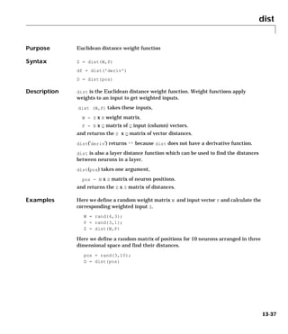

![dlogsig
Purpose Log sigmoid transfer derivative function
dlogsig
Syntax dA_dN = dlogsig(N,A)
Description dlogsig is the derivative function for logsig.
dlogsig(N,A) takes two arguments,
N - S x Q net input.
A - S x Q output.
and returns the S x Q derivative dA/dN.
Examples Here we define the net input N for a layer of 3 tansig neurons.
N = [0.1; 0.8; -0.7];
We calculate the layer's output A with logsig and then the derivative of A with
respect to N.
A = logsig(N)
dA_dN = dlogsig(N,A)
Algorithm The derivative of logsig is calculated as follows:
d = a * (1 - a)
See Also logsig, tansig, dtansig
13-39](https://image.slidesharecdn.com/nnet-090922002848-phpapp01/85/Neural-Network-Toolbox-MATLAB-441-320.jpg)
![dmae
Purpose Mean absolute error performance derivative function
dmae
Syntax dPerf_dE = dmae('e',E,X,perf,PP)
dPerf_dX = dmae('x',E,X,perf,PP)
Description dmae is the derivative function for mae.
dmae('d',E,X,PERF,PP) takes these arguments,
E - Matrix or cell array of error vector(s).
X - Vector of all weight and bias values.
perf - Network performance (ignored).
PP - Performance parameters (ignored).
and returns the derivative dPerf/dE.
dmae('x',E,X,PERF,PP) returns the derivative dPerf/dX.
Examples Here we define E and X for a network with one 3-element output and six weight
and bias values.
E = {[1; -2; 0.5]};
X = [0; 0.2; -2.2; 4.1; 0.1; -0.2];
Here we calculate the network's mean absolute error performance, and
derivatives of performance.
perf = mae(E)
dPerf_dE = dmae('e',E,X)
dPerf_dX = dmae('x',E,X)
Note that mae can be called with only one argument and dmae with only three
arguments because the other arguments are ignored. The other arguments
exist so that mae and dmae conform to standard performance function argument
lists.
See Also mae
13-40](https://image.slidesharecdn.com/nnet-090922002848-phpapp01/85/Neural-Network-Toolbox-MATLAB-442-320.jpg)
![dmse
Purpose Mean squared error performance derivatives function
dmse
Syntax dPerf_dE = dmse('e',E,X,perf,PP)
dPerf_dX = dmse('x',E,X,perf,PP)
Description dmse is the derivative function for mse.
dmse('d',E,X,PERF,PP) takes these arguments,
E - Matrix or cell array of error vector(s).
X - Vector of all weight and bias values.
perf - Network performance (ignored).
PP - Performance parameters (ignored).
and returns the derivative dPerf/dE.
dmse('x',E,X,PERF,PP) returns the derivative dPerf/dX.
Examples Here we define E and X for a network with one 3-element output and six weight
and bias values.
E = {[1; -2; 0.5]};
X = [0; 0.2; -2.2; 4.1; 0.1; -0.2];
Here we calculate the network's mean squared error performance, and
derivatives of performance.
perf = mse(E)
dPerf_dE = dmse('e',E,X)
dPerf_dX = dmse('x',E,X)
Note that mse can be called with only one argument and dmse with only three
arguments because the other arguments are ignored. The other arguments
exist so that mse and dmse conform to standard performance function argument
lists.
See Also mse
13-41](https://image.slidesharecdn.com/nnet-090922002848-phpapp01/85/Neural-Network-Toolbox-MATLAB-443-320.jpg)
![dmsereg
Purpose Mean squared error w/reg performance derivative function
dmsereg
Syntax dPerf_dE = dmsereg('e',E,X,perf,PP)
dPerf_dX = dmsereg('x',E,X,perf,PP)
Description dmsereg is the derivative function for msereg.
dmsereg('d',E,X,PERF,PP) takes these arguments,
E - Matrix or cell array of error vector(s).
X - Vector of all weight and bias values.
perf - Network performance (ignored).
PP - mse performance parameter.
where PP defines one performance parameters,
PP.ratio - Relative importance of errors vs. weight and bias values.
and returns the derivative dPerf/dE.
dmsereg('x',E,X,perf) returns the derivative dPerf/dX.
mse has only one performance parameter.
Examples Here we define an error E and X for a network with one 3-element output and
six weight and bias values.
E = {[1; -2; 0.5]};
X = [0; 0.2; -2.2; 4.1; 0.1; -0.2];
Here the ratio performance parameter is defined so that squared errors are 5
times as important as squared weight and bias values.
pp.ratio = 5/(5+1);
Here we calculate the network's performance, and derivatives of performance.
perf = msereg(E,X,pp)
dPerf_dE = dmsereg('e',E,X,perf,pp)
dPerf_dX = dmsereg('x',E,X,perf,pp)
See Also msereg
13-42](https://image.slidesharecdn.com/nnet-090922002848-phpapp01/85/Neural-Network-Toolbox-MATLAB-444-320.jpg)
![dnetprod
Purpose Derivative of net input product function
dnetprod
Syntax dN_dZ = dnetprod(Z,N)
Description dnetprod is the net input derivative function for netprod.
dnetprod takes two arguments,
Z - S x Q weighted input.
N - S x Q net input.
and returns the S x Q derivative dN/dZ.
Examples Here we define two weighted inputs for a layer with three neurons.
Z1 = [0; 1; -1];
Z2 = [1; 0.5; 1.2];
We calculate the layer's net input N with netprod and then the derivative of N
with respect to each weighted input.
N = netprod(Z1,Z2)
dN_dZ1 = dnetprod(Z1,N)
dN_dZ2 = dnetprod(Z2,N)
Algorithm The derivative a product with respect to any element of that product is the
product of the other elements.
See Also netsum, netprod, dnetsum
13-43](https://image.slidesharecdn.com/nnet-090922002848-phpapp01/85/Neural-Network-Toolbox-MATLAB-445-320.jpg)
![dnetsum
Purpose Sum net input derivative function
dnetsum
Syntax dN_dZ = dnetsum(Z,N)
Description dnetsum is the net input derivative function for netsum.
dnetsum takes two arguments,
Z - S x Q weighted input.
N - S x Q net input.
and returns the S x Q derivative dN/dZ.
Examples Here we define two weighted inputs for a layer with three neurons.
Z1 = [0; 1; -1];
Z2 = [1; 0.5; 1.2];
We calculate the layer's net input N with netsum and then the derivative of N
with respect to each weighted input.
N = netsum(Z1,Z2)
dN_dZ1 = dnetsum(Z1,N)
dN_dZ2 = dnetsum(Z2,N)
Algorithm The derivative of a sum with respect to any element of that sum is always a
ones matrix that is the same size as the sum.
See Also netsum, netprod, dnetprod
13-44](https://image.slidesharecdn.com/nnet-090922002848-phpapp01/85/Neural-Network-Toolbox-MATLAB-446-320.jpg)
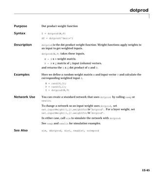
![dposlin
Purpose Derivative of positive linear transfer function
dposlin
Syntax dA_dN = dposlin(N,A)
Description dposlin is the derivative function for poslin.
dposlin(N,A) takes two arguments, and returns the S x Q derivative dA/dN.
Examples Here we define the net input N for a layer of 3 poslin neurons.
N = [0.1; 0.8; -0.7];
We calculate the layer's output A with poslin and then the derivative of A with
respect to N.
A = poslin(N)
dA_dN = dposlin(N,A)
Algorithm The derivative of poslin is calculated as follows:
d = 1, if 0 <= n; 0, Otherwise..
See Also poslin
13-46](https://image.slidesharecdn.com/nnet-090922002848-phpapp01/85/Neural-Network-Toolbox-MATLAB-448-320.jpg)
![dpurelin
Purpose Linear transfer derivative function
dpurelin
Syntax dA_dN = dpurelin(N,A)
Description dpurelin is the derivative function for logsig.
dpurelin(N,A) takes two arguments,
N - S x Q net input.
A - S x Q output.
and returns the S x Q derivative dA_dN.
Examples Here we define the net input N for a layer of 3 purelin neurons.
N = [0.1; 0.8; -0.7];
We calculate the layer's output A with purelin and then the derivative of A
with respect to N.
A = purelin(N)
dA_dN = dpurelin(N,A)
Algorithm The derivative of purelin is calculated as follows:
D(i,q) = 1
See Also purelin
13-47](https://image.slidesharecdn.com/nnet-090922002848-phpapp01/85/Neural-Network-Toolbox-MATLAB-449-320.jpg)
![dradbas
Purpose Derivative of radial basis transfer function
dradbas
Syntax dA_dN = dradbas(N,A)
Description dradbas is the derivative function for radbas.
dradbas(N,A) takes two arguments,
N - S x Q net input.
A - S x Q output.
and returns the S x Q derivative dA/dN.
Examples Here we define the net input N for a layer of 3 radbas neurons.
N = [0.1; 0.8; -0.7];
We calculate the layer's output A with radbas and then the derivative of A with
respect to N.
A = radbas(N)
Algorithm The derivative of radbas is calculated as follows:
d = -2*n*a
See Also radbas
13-48](https://image.slidesharecdn.com/nnet-090922002848-phpapp01/85/Neural-Network-Toolbox-MATLAB-450-320.jpg)
![dsatlin
Purpose Derivative of saturating linear transfer function
dsatlin
Syntax dA_dN = dsatlin(N,A)
Description dsatlin is the derivative function for satlin.
dsatlin(N,A) takes two arguments,
N - S x Q net input.
A - S x Q output.
and returns the S x Q derivative dA/dN.
Examples Here we define the net input N for a layer of 3 satlin neurons.
N = [0.1; 0.8; -0.7];
We calculate the layer's output A with satlin and then the derivative of A with
respect to N.
A = satlin(N)
dA_dN = dsatlin(N,A)
Algorithm The derivative of satlin is calculated as follows:
d = 1, if 0 <= n <= 1; 0, Otherwise..
See Also satlin
13-49](https://image.slidesharecdn.com/nnet-090922002848-phpapp01/85/Neural-Network-Toolbox-MATLAB-451-320.jpg)
![dsatlins
Purpose Derivative of symmetric saturating linear transfer function
dsatlins
Syntax dA_dN = dsatlins(N,A)
Description dsatlins is the derivative function for satlins.
dsatlins(N,A) takes two arguments,
N - S x Q net input.
A - S x Q output.
and returns the S x Q derivative dA/dN.
Examples Here we define the net input N for a layer of 3 satlins neurons.
N = [0.1; 0.8; -0.7];
We calculate the layer's output A with satlins and then the derivative of A
with respect to N.
A = satlins(N)
dA_dN = dsatlins(N,A)
Algorithm The derivative of satlins is calculated as follows:
d = 1, if -1 <= n <= 1; 0, Otherwise.
See Also satlins
13-50](https://image.slidesharecdn.com/nnet-090922002848-phpapp01/85/Neural-Network-Toolbox-MATLAB-452-320.jpg)
![dsse
Purpose Sum squared error performance derivative function
dsse
Syntax dPerf_dE = dsse('e',E,X,perf,PP)
dPerf_dX = dsse('x',E,X,perf,PP)
Description dsse is the derivative function for sse.
dsse('d',E,X,perf,PP) takes these arguments,
E - Matrix or cell array of error vector(s).
X - Vector of all weight and bias values.
perf - Network performance (ignored).
PP - Performance parameters (ignored).
and returns the derivative dPerf_dE.
dsse('x',E,X,perf,PP)returns the derivative dPerf_dX.
Examples Here we define an error E and X for a network with one 3-element output and
six weight and bias values.
E = {[1; -2; 0.5]};
X = [0; 0.2; -2.2; 4.1; 0.1; -0.2];
Here we calculate the network's sum squared error performance, and
derivatives of performance.
perf = sse(E)
dPerf_dE = dsse('e',E,X)
dPerf_dX = dsse('x',E,X)
Note that sse can be called with only one argument and dsse with only three
arguments because the other arguments are ignored. The other arguments
exist so that sse and dsse conform to standard performance function argument
lists.
See Also sse
13-51](https://image.slidesharecdn.com/nnet-090922002848-phpapp01/85/Neural-Network-Toolbox-MATLAB-453-320.jpg)
![dtansig
Purpose Hyperbolic tangent sigmoid transfer derivative function
dtansig
Syntax dA_dN = dtansig(N,A)
Description dtansig is the derivative function for tansig.
dtansig(N,A) takes two arguments,
N - S x Q net input.
A - S x Q output.
and returns the S x Q derivative dA/dN.
Examples Here we define the net input N for a layer of 3 tansig neurons.
N = [0.1; 0.8; -0.7];
We calculate the layer's output A with tansig and then the derivative of A with
respect to N.
A = tansig(N)
dA_dN = dtansig(N,A)
Algorithm The derivative of tansig is calculated as follows:
d = 1-a^2
See Also tansig, logsig, dlogsig
13-52](https://image.slidesharecdn.com/nnet-090922002848-phpapp01/85/Neural-Network-Toolbox-MATLAB-454-320.jpg)
![dtribas
Purpose Derivative of triangular basis transfer function
dtribas
Syntax dA_dN = dtribas(N,A)
Description dtribas is the derivative function for tribas.
dtribas(N,A) takes two arguments,
N - S x Q net input.
A - S x Q output.
and returns the S x Q derivative dA/dN.
Examples Here we define the net input N for a layer of 3 tribas neurons.
N = [0.1; 0.8; -0.7];
We calculate the layer's output A with tribas and then the derivative of A with
respect to N.
A = tribas(N)
dA_dN = dtribas(N,A)
Algorithm The derivative of tribas is calculated as follows:
d = 1, if -1 <= n < 0; -1, if 0 < n <= 1; 0, Otherwise.
See Also tribas
13-53](https://image.slidesharecdn.com/nnet-090922002848-phpapp01/85/Neural-Network-Toolbox-MATLAB-455-320.jpg)
![errsurf
Purpose Error surface of single input neuron
errsurf
Syntax errsurf(p,t,wv,bv,f)
Description errsurf(p,t,wv,bv,f) takes these arguments,
P - 1 x Q matrix of input vectors.
T - 1 x Q matrix of target vectors.
WV - Row vector of values of W.
BV - Row vector of values of B.
F - Transfer function (string).
and returns a matrix of error values over WV and BV.
Examples p = [-6.0 -6.1 -4.1 -4.0 +4.0 +4.1 +6.0 +6.1];
t = [+0.0 +0.0 +.97 +.99 +.01 +.03 +1.0 +1.0];
wv = -1:.1:1; bv = -2.5:.25:2.5;
es = errsurf(p,t,wv,bv,'logsig');
plotes(wv,bv,ES,[60 30])
See Also plotes
13-54](https://image.slidesharecdn.com/nnet-090922002848-phpapp01/85/Neural-Network-Toolbox-MATLAB-456-320.jpg)
![gensim
Purpose Generate a simulink block for neural network simulation
gensim
Syntax gensim(net,st)
To Get Help Type help network/gensim
Description gensim(net,st) creates a simulink system containing a block which simulates
neural network net.
gensim(net,st) takes these inputs,
net - Neural network.
st - Sample time (default = 1).
and creates a Simulink system containing a block which simulates neural
network net with a sampling time of st.
If net has no input or layer delays (net.numInputDelays and
net.numLayerDelays are both 0) then you can use -1 for st to get a
continuously sampling network.
Examples net = newff([0 1],[5 1]);
gensim(net)
13-55](https://image.slidesharecdn.com/nnet-090922002848-phpapp01/85/Neural-Network-Toolbox-MATLAB-457-320.jpg)

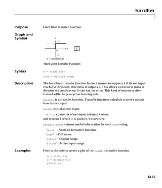

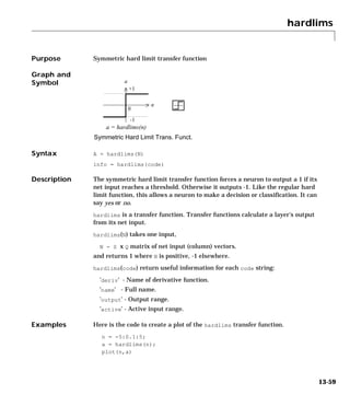

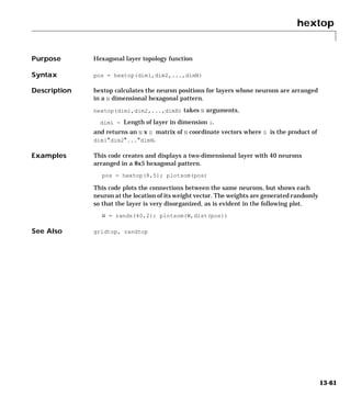
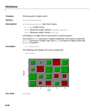
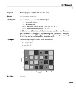
![ind2vec
Purpose Convert indices to vectors
ind2vec
Syntax vec = ind2vec(ind)
Description ind2vec and vec2ind allow indices to either be represented by themselves, or
as vectors containing a 1 in the row of the index they represent.
ind2vec(ind) takes one argument,
ind - Row vector of indices.
and returns a sparse matrix of vectors, with one 1 in each column, as indicated
by ind.
Examples Here four indices are defined and converted to vector representation.
ind = [1 3 2 3]
vec = ind2vec(ind)
See Also vec2ind
13-64](https://image.slidesharecdn.com/nnet-090922002848-phpapp01/85/Neural-Network-Toolbox-MATLAB-466-320.jpg)
![init
Purpose Initialize a neural network
init
Syntax net = init(net)
To Get Help Type help network/init
Description init(net) returns neural network net with weight and bias values updated
according to the network initialization function, indicated by net.initFcn,
and the parameter values, indicated by net.initParam.
Examples Here a perceptron is created with a 2-element input (with ranges of 0 to 1, and
-2 to 2) and 1 neuron. Once it is created we can display the neuron’s weights
and bias.
net = newp([0 1;-2 2],1);
net.iw{1,1}
net.b{1}
Training the perceptron alters its weight and bias values.
P = [0 1 0 1; 0 0 1 1];
T = [0 0 0 1];
net = train(net,P,T);
net.iw{1,1}
net.b{1}
init reinitializes those weight and bias values.
net = init(net);
net.iw{1,1}
net.b{1}
The weights and biases are zeros again, which are the initial values used by
perceptron networks (see newp).
Algorithm init calls net.initFcn to initialize the weight and bias values according to the
parameter values net.initParam.
Typically, net.initFcn is set to 'initlay' which initializes each layer's
weights and biases according to its net.layers{i}.initFcn.
13-65](https://image.slidesharecdn.com/nnet-090922002848-phpapp01/85/Neural-Network-Toolbox-MATLAB-467-320.jpg)

![initcon
Purpose Conscience bias initialization function
initcon
Syntax b = initcon(s,pr)
Description initcon is a bias initialization function that initializes biases for learning with
the learncon learning function.
initcon (S,PR) takes two arguments,
S - Number of rows (neurons).
PR - R x 2 matrix of R = [Pmin Pmax], default = [1 1].
and returns an S x 1 bias vector.
Note that for biases R is always 1. initcon could also be used to initialize
weights, but it is not recommended for that purpose.
Examples Here initial bias values are calculated for a 5 neuron layer.
b = initcon(5)
Network Use You can create a standard network that uses initcon to initialize weights by
calling newc.
To prepare the bias of layer i of a custom network to initialize with initcon:
1 Set net.initFcn to 'initlay'. (net.initParam will automatically become
initlay's default parameters.)
2 Set net.layers{i}.initFcn to 'initwb'.
3 Set net.biases{i}.initFcn to 'initcon'.
To initialize the network call init. See newc for initialization examples.
Algorithm learncon updates biases so that each bias value b(i) is a function of the
average output c(i) of the neuron i associated with the bias.
initcon gets initial bias values by assuming that each neuron has responded
to equal numbers of vectors in the "past".
See Also initwb, initlay, init, learncon
13-67](https://image.slidesharecdn.com/nnet-090922002848-phpapp01/85/Neural-Network-Toolbox-MATLAB-469-320.jpg)
![initlay
Purpose Layer-by-layer network initialization function
initlay
Syntax net = initlay(net)
info = initlay(code)
Description initlay is a network initialization function which initializes each layer i
according to its own initialization function net.layers{i}.initFcn.
initlay(net) takes,
net - Neural network.
and returns the network with each layer updated. initlay(code) returns
useful information for each code string:
'pnames' - Names of initialization parameters.
'pdefaults' - Default initialization parameters.
initlay does not have any initialization parameters.
Network Use You can create a standard network that uses initlay by calling newp, newlin,
newff, newcf, and many other new network functions.
To prepare a custom network to be initialized with initlay:
1 Set net.initFcn to 'initlay'. (This will set net.initParam to the empty
matrix [ ] since initlay has no initialization parameters.)
2 Set each net.layers{i}.initFcn to a layer initialization function.
(Examples of such functions are initwb and initnw).
To initialize the network call init. See newp and newlin for initialization
examples.
Algorithm The weights and biases of each layer i are initialized according to
net.layers{i}.initFcn.
See Also initwb, initnw, init
13-68](https://image.slidesharecdn.com/nnet-090922002848-phpapp01/85/Neural-Network-Toolbox-MATLAB-470-320.jpg)
![initnw
Purpose Nguyen-Widrow layer initialization function
initnw
Syntax net = initnw(net,i)
Description initnw is a layer initialization function which initializes a layer's weights and
biases according to the Nguyen-Widrow initialization algorithm. This
algorithm chooses values in order to distribute the active region of each neuron
in the layer evenly across the layer's input space.
initnw(net,i) takes two arguments,
net - Neural network.
i - Index of a layer.
and returns the network with layer i's weights and biases updated.
Network Use You can create a standard network that uses initnw by calling newff or newcf.
To prepare a custom network to be initialized with initnw:
1 Set net.initFcn to 'initlay'. (This will set net.initParam to the empty
matrix [ ] since initlay has no initialization parameters.)
2 Set net.layers{i}.initFcn to 'initnw'.
To initialize the network call init. See newff and newcf for training examples.
Algorithm The Nguyen-Widrow method generates initial weight and bias values for a
layer, so that the active regions of the layer's neurons will be distributed
roughly evenly over the input space.
Advantages over purely random weights and biases are:
1 Few neurons are wasted (since all the neurons are in the input space).
2 Training works faster (since each area of the input space has neurons). The
Nguyen-Widrow method can only be applied to layers...
- with a bias,
- with weights whose "weightFcn" is dotprod,
- with "netInputFcn" set to netsum.
If these conditions are not met then initnw uses rands to initialize the layer's
weights and biases.
See Also initwb, initlay, init
13-69](https://image.slidesharecdn.com/nnet-090922002848-phpapp01/85/Neural-Network-Toolbox-MATLAB-471-320.jpg)
![initwb
Purpose By-weight-and-bias layer initialization function
initwb
Syntax net = initwb(net,i)
Description initwb is a layer initialization function with initializes a layer's weights and
biases according to their own initialization functions.
initwb(net,i) takes two arguments,
net - Neural network.
i - Index of a layer.
and returns the network with layer i's weights and biases updated.
Network Use You can create a standard network that uses initwb by calling newp or newlin.
To prepare a custom network to be initialized with initwb:
1 Set net.initFcn to 'initlay'. (This will set net.initParam to the empty
matrix [ ] since initlay has no initialization parameters.)
2 Set net.layers{i}.initFcn to 'initwb'.
3 Set each net.inputWeights{i,j}.learnFcn to a weight initialization
function. Set each net.layerWeights{i,j}.learnFcn to a weight
initialization function. Set each net.biases{i}.learnFcn to a bias
initialization function. (Examples of such functions are rands and
midpoint.)
To initialize the network call init.
See newp and newlin for training examples.
Algorithm Each weight (bias) in layer i is set to new values calculated according to its
weight (bias) initialization function.
See Also initnw, initlay, init
13-70](https://image.slidesharecdn.com/nnet-090922002848-phpapp01/85/Neural-Network-Toolbox-MATLAB-472-320.jpg)
![initzero
Purpose Zero weight/bias initialization function
initzero
Syntax W = initzero(S,PR)
b = initzero(S,[1 1])
Description initzero(S,PR) takes two arguments,
S - Number of rows (neurons).
PR - R x 2 matrix of input value ranges = [Pmin Pmax].
and returns an S x R weight matrix of zeros.
initzero(S,[1 1]) returns S x 1 bias vector of zeros.
Examples Here initial weights and biases are calculated for a layer with two inputs
ranging over [0 1] and [-2 2], and 4 neurons.
W = initzero(5,[0 1; -2 2])
b = initzero(5,[1 1])
Network Use You can create a standard network that uses initzero to initialize its weights
by calling newp or newlin.
To prepare the weights and the bias of layer i of a custom network to be
initialized with midpoint:
1 Set net.initFcn to 'initlay'. (net.initParam will automatically become
initlay's default parameters.)
2 Set net.layers{i}.initFcn to 'initwb'.
3 Set each net.inputWeights{i,j}.initFcn to 'initzero'. Set each
net.layerWeights{i,j}.initFcn to 'initzero'. Set each
net.biases{i}.initFcn to 'initzero'.
To initialize the network call init.
See newp or newlin for initialization examples.
See Also initwb, initlay, init
13-71](https://image.slidesharecdn.com/nnet-090922002848-phpapp01/85/Neural-Network-Toolbox-MATLAB-473-320.jpg)
![learncon
Purpose Conscience bias learning function
learncon
Syntax [dB,LS] = learncon(B,P,Z,N,A,T,E,gW,gA,D,LP,LS)
info = learncon(code)
Description learncon is the conscience bias learning function used to increase the net input
to neurons which have the lowest average output until each neuron responds
roughly an equal percentage of the time.
learncon(B,P,Z,N,A,T,E,gW,gA,D,LP,LS) takes several inputs,
B - S x 1 bias vector.
P - 1x Q ones vector.
Z - S x Q weighted input vectors.
N - S x Q net input vectors.
A - S x Q output vectors.
T - S x Q layer target vectors.
E - S x Q layer error vectors.
gW - S x R gradient with respect to performance.
gA - S x Q output gradient with respect to performance.
D - S x S neuron distances.
LP - Learning parameters, none, LP = [].
LS - Learning state, initially should be = [].
and returns
dB - S x 1 weight (or bias) change matrix.
LS - New learning state.
Learning occurs according to learncon's learning parameter, shown here with
its default value.
LP.lr - 0.001 - Learning rate.
learncon(code) returns useful information for each code string,
'pnames' - Names of learning parameters.
'pdefaults' - Default learning parameters.
'needg' - Returns 1 if this function uses gW or gA.
NNT 2.0 compatibility: The LP.lr described above equals 1 minus the bias time
constant used by trainc in NNT 2.0.
13-72](https://image.slidesharecdn.com/nnet-090922002848-phpapp01/85/Neural-Network-Toolbox-MATLAB-474-320.jpg)
![learncon
Examples Here we define a random output A, and bias vector W for a layer with 3 neurons.
We also define the learning rate LR.
a = rand(3,1);
b = rand(3,1);
lp.lr = 0.5;
Since learncon only needs these values to calculate a bias change (see
algorithim below), we will use them to do so.
dW = learncon(b,[],[],[],a,[],[],[],[],[],lp,[])
Network Use To prepare the bias of layer i of a custom network to learn with learncon:
1 Set net.trainFcn to 'trainwb1'. (net.trainParam will automatically
become adaptwb's default parameters.)
2 Set net.adaptFcn to 'adaptwb'. (net.adaptParam will automatically become
adaptwb's default parameters.)
3 Set net.inputWeights{i}.learnFcn to 'learncon'. Set each
net.layerWeights{i,j}.learnFcn to 'learncon'. (Each weight learning
parameter property will automatically be set to learncon's default
parameters.)
To train the network (or enable it to adapt):
1 Set net.trainParam (or net.adaptParam) properties as desired.
2 Call train (or adapt).
Algorithm learncon calculates the bias change db for a given neuron by first updating
each neuron's conscience, i.e. the running average of its output:
c = (1-lr)*c + lr*a
The conscience is then used to compute a bias for the neuron that is greatest
for smaller conscience values.
b = exp(1-log(c)) - b
(Note that learncon is able to recover C each time it is called from the bias
values.)
See Also learnk, learnos, adaptwb, trainwb, adapt, train
13-73](https://image.slidesharecdn.com/nnet-090922002848-phpapp01/85/Neural-Network-Toolbox-MATLAB-475-320.jpg)
![learngd
Purpose Gradient descent weight/bias learning function
learngd
Syntax [dW,LS] = learngd(W,P,Z,N,A,T,E,gW,gA,D,LP,LS)
[db,LS] = learngd(b,ones(1,Q),Z,N,A,T,E,gW,gA,D,LP,LS)
info = learngd(code)
Description learngd is the gradient descent weight/bias learning function.
learngd(W,P,Z,N,A,T,E,gW,gA,D,LP,LS) takes several inputs,
W - S x R weight matrix (or S x 1 bias vector).
P - R x Q input vectors (or ones(1,Q)).
Z - S x Q weighted input vectors.
N - S x Q net input vectors.
A - S x Q output vectors.
T - S x Q layer target vectors.
E - S x Q layer error vectors.
gW - S x R gradient with respect to performance.
gA - S x Q output gradient with respect to performance.
D - S x S neuron distances.
LP - Learning parameters, none, LP = [].
LS - Learning state, initially should be = [].
and returns,
dW - S x R weight (or bias) change matrix.
LS - New learning state.
Learning occurs according to learngd's learning parameter shown here with
its default value.
LP.lr - 0.01 - Learning rate.
learngd(code) returns useful information for each code string:
'pnames' - Names of learning parameters.
'pdefaults' - Default learning parameters.
'needg' - Returns 1 if this function uses gW or gA.
13-74](https://image.slidesharecdn.com/nnet-090922002848-phpapp01/85/Neural-Network-Toolbox-MATLAB-476-320.jpg)
![learngd
Examples Here we define a random gradient gW for a weight going to a layer with 3
neurons, from an input with 2 elements. We also define a learning rate of 0.5.
gW = rand(3,2);
lp.lr = 0.5;
Since learngd only needs these values to calculate a weight change (see
algorithim below), we will use them to do so.
dW = learngd([],[],[],[],[],[],[],gW,[],[],lp,[])
Network Use You can create a standard network that uses learngd with newff, newcf, or
newelm. To prepare the weights and the bias of layer i of a custom network to
adapt with learngd:
1 Set net.adaptFcn to 'adaptwb'. net.adaptParam will automatically become
trainwb's default parameters.
2 Set each net.inputWeights{i,j}.learnFcn to 'learngd'. Set each
net.layerWeights{i,j}.learnFcn to 'learngd'. Set
net.biases{i}.learnFcn to 'learngd'. Each weight and bias learning
parameter property will automatically be set to learngd's default
parameters.
To allow the network to adapt:
1 Set net.adaptParam properties to desired values.
2 Call adapt with the network.
See newff or newcf for examples.
Algoritm learngd calculates the weight change dW for a given neuron from the neuron's
input P and error E, and the weight (or bias) learning rate LR, according to the
gradient descent: dw = lr*gW.
See Also learngdm, newff, newcf, adaptwb, trainwb, adapt, train
13-75](https://image.slidesharecdn.com/nnet-090922002848-phpapp01/85/Neural-Network-Toolbox-MATLAB-477-320.jpg)
![learngdm
Purpose Gradient descent w/ momentum weight/bias learning function
learngdm
Syntax [dW,LS] = learngdm(W,P,Z,N,A,T,E,gW,gA,D,LP,LS)
[db,LS] = learngdm(b,ones(1,Q),Z,N,A,T,E,gW,gA,D,LP,LS)
info = learngdm(code)
Description learngdm is the gradient descent with momentum weight/bias learning
function.
learngdm(W,P,Z,N,A,T,E,gW,gA,D,LP,LS) takes several inputs,
W - S x R weight matrix (or S x 1 bias vector).
P - R x Q input vectors (or ones(1,Q)).
Z - S x Q weighted input vectors.
N - S x Q net input vectors.
A - S x Q output vectors.
T - S x Q layer target vectors.
E - S x Q layer error vectors.
gW - S x R gradient with respect to performance.
gA - S x Q output gradient with respect to performance.
D - S x S neuron distances.
LP - Learning parameters, none, LP = [].
LS - Learning state, initially should be = [].
and returns,
dW - S x R weight (or bias) change matrix.
LS - New learning state.
Learning occurs according to learngdm's learning parameters, shown here with
their default values.
LP.lr - 0.01 - Learning rate.
LP.mc - 0.9 - Momentum constant.
13-76](https://image.slidesharecdn.com/nnet-090922002848-phpapp01/85/Neural-Network-Toolbox-MATLAB-478-320.jpg)
![learngdm
learngdm(code) returns useful information for each code string:
'pnames' - Names of learning parameters.
'pdefaults' - Default learning parameters.
'needg' - Returns 1 if this function uses gW or gA.
Examples Here we define a random gradient G for a weight going to a layer with 3
neurons, from an input with 2 elements. We also define a learning rate of 0.5
and momentum constant of 0.8;
gW = rand(3,2);
lp.lr = 0.5;
lp.mc = 0.8;
Since learngdm only needs these values to calculate a weight change (see
algorithim below), we will use them to do so. We will use the default initial
learning state.
ls = [];
[dW,ls] = learngdm([],[],[],[],[],[],[],gW,[],[],lp,ls)
learngdm returns the weight change and a new learning state.
Network Use You can create a standard network that uses learngdm with newff, newcf, or newelm.
To prepare the weights and the bias of layer i of a custom network to adapt
with learngdm:
1 Set net.adaptFcn to 'adaptwb'. net.adaptParam will automatically become
trainwb's default parameters.
2 Set each net.inputWeights{i,j}.learnFcn to 'learngdm'. Set each
net.layerWeights{i,j}.learnFcn to 'learngdm'. Set
net.biases{i}.learnFcn to 'learngdm'. Each weight and bias learning
parameter property will automatically be set to learngdm's default
parameters.
To allow the network to adapt:
1 Set net.adaptParam properties to desired values.
2 Call adapt with the network.
See newff or newcf for examples.
13-77](https://image.slidesharecdn.com/nnet-090922002848-phpapp01/85/Neural-Network-Toolbox-MATLAB-479-320.jpg)

![learnh
Purpose Hebb weight learning rule
learnh
Syntax [dW,LS] = learnh(W,P,Z,N,A,T,E,gW,gA,D,LP,LS)
info = learnh(code)
Description learnh is the Hebb weight learning function.
learnh(W,P,Z,N,A,T,E,gW,gA,D,LP,LS) takes several inputs,
W - S x R weight matrix (or S x 1 bias vector).
P - R x Q input vectors (or ones(1,Q)).
Z - S x Q weighted input vectors.
N - S x Q net input vectors.
A - S x Q output vectors.
T - S x Q layer target vectors.
E - S x Q layer error vectors.
gW - S x R gradient with respect to performance.
gA - S x Q output gradient with respect to performance.
D - S x S neuron distances.
LP - Learning parameters, none, LP = [].
LS - Learning state, initially should be = [].
and returns,
dW - S x R weight (or bias) change matrix.
LS - New learning state.
Learning occurs according to learnh's learning parameter, shown here with its
default value.
LP.lr - 0.01 - Learning rate.
learnh(code) returns useful information for each code string:
'pnames' - Names of learning parameters.
'pdefaults' - Default learning parameters.
'needg' - Returns 1 if this function uses gW or gA.
13-79](https://image.slidesharecdn.com/nnet-090922002848-phpapp01/85/Neural-Network-Toolbox-MATLAB-481-320.jpg)
![learnh
Examples Here we define a random input P and output A for a layer with a 2-element
input and 3 neurons. We also define the learning rate LR.
p = rand(2,1);
a = rand(3,1);
lp.lr = 0.5;
Since learnh only needs these values to calculate a weight change (see
algorithim below), we will use them to do so.
dW = learnh([],p,[],[],a,[],[],[],[],[],lp,[])
Network Use To prepare the weights and the bias of layer i of a custom network to learn with
learnh:
1 Set net.trainFcn to 'trainwb'. (net.trainParam will automatically become
trainwb's default parameters.)
2 Set net.adaptFcn to 'adaptwb'. (net.adaptParam will automatically become
trainwb's default parameters.)
3 Set each net.inputWeights{i,j}.learnFcn to 'learnh'. Set each
net.layerWeights{i,j}.learnFcn to 'learnh'. Each weight learning
parameter property will automatically be set to learnh's default
parameters.)
To train the network (or enable it to adapt):
1 Set net.trainParam (net.adaptParam) properties to desired values.
2 Call train (adapt).
Algorithm learnh calculates the weight change dW for a given neuron from the neuron's
input P, output A, and learning rate LR according to the Hebb learning rule:
dw = lr*a*p'
See Also learnhd, adaptwb, trainwb, adapt, train
References Hebb, D.O., The Organization of Behavior, New York: Wiley, 1949.
13-80](https://image.slidesharecdn.com/nnet-090922002848-phpapp01/85/Neural-Network-Toolbox-MATLAB-482-320.jpg)
![learnhd
Purpose Hebb with decay weight learning rule
learnhd
Syntax [dW,LS] = learnhd(W,P,Z,N,A,T,E,gW,gA,D,LP,LS)
info = learnhd(code)
Description learnhd is the Hebb weight learning function.
learnhd(W,P,Z,N,A,T,E,gW,gA,D,LP,LS) takes several inputs,
W - S x R weight matrix (or S x 1 bias vector).
P - R x Q input vectors (or ones(1,Q)).
Z - S x Q weighted input vectors.
N - S x Q net input vectors.
A - S x Q output vectors.
T - S x Q layer target vectors.
E - S x Q layer error vectors.
gW - S x R gradient with respect to performance.
gA - S x Q output gradient with respect to performance.
D - S x S neuron distances.
LP - Learning parameters, none, LP = [].
LS - Learning state, initially should be = [].
and returns,
dW - S x R weight (or bias) change matrix.
LS - New learning state.
Learning occurs according to learnhd's learning parameters shown here with
default values.
LP.dr - 0.01 - Decay rate.
LP.lr - 0.1 - Learning rate.
learnhd(code) returns useful information for each code string:
'pnames' - Names of learning parameters.
'pdefaults' - Default learning parameters.
'needg' - Returns 1 if this function uses gW or gA.
13-81](https://image.slidesharecdn.com/nnet-090922002848-phpapp01/85/Neural-Network-Toolbox-MATLAB-483-320.jpg)
![learnhd
Examples Here we define a random input P, output A, and weights W for a layer with a
2-element input and 3 neurons. We also define the decay and learning rates.
p = rand(2,1);
a = rand(3,1);
w = rand(3,2);
lp.dr = 0.05;
lp.lr = 0.5;
Since learnhd only needs these values to calculate a weight change (see
algorithm below), we will use them to do so.
dW = learnhd(w,p,[],[],a,[],[],[],[],[],lp,[])
Network Use To prepare the weights and the bias of layer i of a custom network to learn with
learnhd:
1 Set net.trainFcn to 'trainwb'. (net.trainParam will automatically become
trainwb's default parameters.)
2 Set net.adaptFcn to 'adaptwb'. (net.adaptParam will automatically become
trainwb's default parameters.)
3 Set each net.inputWeights{i,j}.learnFcn to 'learnhd'. Set each
net.layerWeights{i,j}.learnFcn to 'learnhd'. (Each weight learning
parameter property will automatically be set to learnhd's default
parameters.)
To train the network (or enable it to adapt):
1 Set net.trainParam (net.adaptParam) properties to desired values.
2 Call train (adapt).
Algorithm learnhd calculates the weight change dW for a given neuron from the neuron's
input P, output A, decay rate DR, and learning rate LR according to the Hebb
with decay learning rule:
dw = lr*a*p' - dr*w
See Also learnh, adaptwb, trainwb, adapt, train
13-82](https://image.slidesharecdn.com/nnet-090922002848-phpapp01/85/Neural-Network-Toolbox-MATLAB-484-320.jpg)
![learnis
Purpose Instar weight learning function
learnis
Syntax [dW,LS] = learnis(W,P,Z,N,A,T,E,gW,gA,D,LP,LS)
info = learnis(code)
Description learnis is the instar weight learning function.
learnis(W,P,Z,N,A,T,E,gW,gA,D,LP,LS) takes several inputs,
W - S x R weight matrix (or S x 1 bias vector).
P - R x Q input vectors (or ones(1,Q)).
Z - S x Q weighted input vectors.
N - S x Q net input vectors.
A - S x Q output vectors.
T - S x Q layer target vectors.
E - S x Q layer error vectors.
gW - S x R gradient with respect to performance.
gA - S x Q output gradient with respect to performance.
D - S x S neuron distances.
LP - Learning parameters, none, LP = [].
LS - Learning state, initially should be = [].
and returns,
dW - S x R weight (or bias) change matrix.
LS - New learning state.
Learning occurs according to learnis's learning parameter, shown here with
its default value.
LP.lr - 0.01 - Learning rate.
learnis(code) return useful information for each code string:
'pnames' - Names of learning parameters.
'pdefaults' - Default learning parameters.
'needg' - Returns 1 if this function uses gW or gA.
13-83](https://image.slidesharecdn.com/nnet-090922002848-phpapp01/85/Neural-Network-Toolbox-MATLAB-485-320.jpg)
![learnis
Examples Here we define a random input P, output A, and weight matrix W for a layer with
a 2-element input and 3 neurons. We also define the learning rate LR.
p = rand(2,1);
a = rand(3,1);
w = rand(3,2);
lp.lr = 0.5;
Since learnis only needs these values to calculate a weight change (see
algorithm below), we will use them to do so.
dW = learnis(w,p,[],[],a,[],[],[],[],[],lp,[])
Network Use To prepare the weights and the bias of layer i of a custom network so that it
can learn with learnis:
1 Set net.trainFcn to 'trainwb'. (net.trainParam will automatically become
trainwb's default parameters.)
2 Set net.adaptFcn to 'adaptwb'. (net.adaptParam will automatically become
trainwb's default parameters.)
3 Set each net.inputWeights{i,j}.learnFcn to 'learnis'. Set each
net.layerWeights{i,j}.learnFcn to 'learnis'. (Each weight learning
parameter property will automatically be set to learnis's default
parameters.)
To train the network (or enable it to adapt):
1 Set net.trainParam (net.adaptParam) properties to desired values.
2 Call train (adapt).
Algorithm learnis calculates the weight change dW for a given neuron from the neuron's
input P, output A, and learning rate LR according to the instar learning rule:
dw = lr*a*(p'-w)
See Also learnk, learnos, adaptwb, trainwb, adapt, train
References Grossberg, S., Studies of the Mind and Brain, Drodrecht, Holland: Reidel
Press, 1982.
13-84](https://image.slidesharecdn.com/nnet-090922002848-phpapp01/85/Neural-Network-Toolbox-MATLAB-486-320.jpg)
![learnk
Purpose Kohonen weight learning function
learnk
Syntax [dW,LS] = learnk(W,P,Z,N,A,T,E,gW,gA,D,LP,LS)
info = learnk(code)
Description learnk is the Kohonen weight learning function.
learnk(W,P,Z,N,A,T,E,gW,gA,D,LP,LS) takes several inputs,
W - S x R weight matrix (or S x 1 bias vector).
P - R x Q input vectors (or ones(1,Q)).
Z - S x Q weighted input vectors.
N - S x Q net input vectors.
A - S x Q output vectors.
T - S x Q layer target vectors.
E - S x Q layer error vectors.
gW - S x R gradient with respect to performance.
gA - S x Q output gradient with respect to performance.
D - S x S neuron distances.
LP - Learning parameters, none, LP = [].
LS - Learning state, initially should be = [].
and returns,
dW - S x R weight (or bias) change matrix.
LS - New learning state.
Learning occurs according to learnk's learning parameter, shown here with its
default value.
LP.lr - 0.01 - Learning rate.
learnk(code) returns useful information for each code string:
'pnames' - Names of learning parameters.
'pdefaults' - Default learning parameters.
'needg' - Returns 1 if this function uses gW or gA.
13-85](https://image.slidesharecdn.com/nnet-090922002848-phpapp01/85/Neural-Network-Toolbox-MATLAB-487-320.jpg)
![learnk
Examples Here we define a random input P, output A, and weight matrix W for a layer with
a 2-element input and 3 neurons. We also define the learning rate LR.
p = rand(2,1);
a = rand(3,1);
w = rand(3,2);
lp.lr = 0.5;
Since learnk only needs these values to calculate a weight change (see
algorithm below), we will use them to do so.
dW = learnk(w,p,[],[],a,[],[],[],[],[],lp,[])
Network Use To prepare the weights of layer i of a custom network to learn with learnk:
1 Set net.trainFcn to 'trainwb1'. (net.trainParam will automatically
become trainwb1's default parameters.)
2 Set net.adaptFcn to 'adaptwb'. (net.adaptParam will automatically become
trainwb1's default parameters.)
3 Set each net.inputWeights{i,j}.learnFcn to 'learnk'. Set each
net.layerWeights{i,j}.learnFcn to 'learnk'. (Each weight learning
parameter property will automatically be set to learnk's default
parameters.)
To train the network (or enable it to adapt):
1 Set net.trainParam (or net.adaptParam) properties as desired.
2 Call train (or adapt).
Algorithm learnk calculates the weight change dW for a given neuron from the neuron's
input P, output A, and learning rate LR according to the Kohonen learning rule:
dw = lr*(p'-w), if a ~= 0; = 0, otherwise.
See Also learnis, learnos, adaptwb, trainwb, adapt, train
References Kohonen, T., Self-Organizing and Associative Memory, New York:
Springer-Verlag, 1984.
13-86](https://image.slidesharecdn.com/nnet-090922002848-phpapp01/85/Neural-Network-Toolbox-MATLAB-488-320.jpg)
![learnlv1
Purpose LVQ1 weight learning function
learnlv1
Syntax [dW,LS] = learnlv1(W,P,Z,N,A,T,E,gW,gA,D,LP,LS)
info = learnlv1(code)
Description learnlv1 is the LVQ1 weight learning function.
learnlv1(W,P,Z,N,A,T,E,gW,gA,D,LP,LS) takes several inputs,
W - S x R weight matrix (or S x 1 bias vector).
P - R x Q input vectors (or ones(1,Q)).
Z - S x Q weighted input vectors.
N - S x Q net input vectors.
A - S x Q output vectors.
T - S x Q layer target vectors.
E - S x Q layer error vectors.
gW - S x R weight gradient with respect to performance.
gA - S x Q output gradient with respect to performance.
D - S x R neuron distances.
LP - Learning parameters, none, LP = [].
LS - Learning state, initially should be = [].
and returns,
dW - S x R weight (or bias) change matrix.
LS - New learning state.
Learning occurs according to learnlv1's learning parameter shown here with
its default value.
LP.lr - 0.01 - Learning rate.
learnlv1(code) returns useful information for each code string:
'pnames' - Names of learning parameters.
'pdefaults' - Default learning parameters.
needg' - Returns 1 if this function uses gW or gA.
13-87](https://image.slidesharecdn.com/nnet-090922002848-phpapp01/85/Neural-Network-Toolbox-MATLAB-489-320.jpg)
![learnlv1
Examples Here we define a random input P, output A, weight matrix W, and output
gradient gA for a layer with a 2-element input and 3 neurons.
We also define the learning rate LR.
p = rand(2,1);
w = rand(3,2);
a = compet(negdist(w,p));
gA = [-1;1; 1];
lp.lr = 0.5;
Since learnlv1 only needs these values to calculate a weight change (see
algorithm below), we will use them to do so.
dW = learnlv1(w,p,[],[],a,[],[],[],gA,[],lp,[])
Network Use You can create a standard network that uses learnlv1 with newlvq. To prepare
the weights of layer i of a custom network to learn with learnlv1:
1 Set net.trainFcn to trainwb1'. (net.trainParam will automatically become
trainwb1's default parameters.)
2 Set net.adaptFcn to 'adaptwb'. (net.adaptParam will automatically become
trainwb1's default parameters.)
3 Set each net.inputWeights{i,j}.learnFcn to 'learnlv1'. Set each
net.layerWeights{i,j}.learnFcn to 'learnlv1'. (Each weight learning
parameter property will automatically be set to learnlv1's default
parameters.)
To train the network (or enable it to adapt):
1 Set net.trainParam (or net.adaptParam) properties as desired.
2 Call train (or adapt).
Algorithm learnlv1 calculates the weight change dW for a given neuron from the neuron's
input P, output A, output gradient gA and learning rate LR, according to the
LVQ1 rule, given i the index of the neuron whose output a(i) is 1:
dw(i,:) = +lr*(p-w(i,:)) if gA(i) = 0;= -lr*(p-w(i,:)) if gA(i) = -1
See Also learnlv2, adaptwb, trainwb, adapt, train
13-88](https://image.slidesharecdn.com/nnet-090922002848-phpapp01/85/Neural-Network-Toolbox-MATLAB-490-320.jpg)
![learnlv2
Purpose LVQ2 weight learning function
learnlv2
Syntax [dW,LS] = learnlv2(W,P,Z,N,A,T,E,gW,gA,D,LP,LS)
info = learnlv2(code)
Description learnlv2 is the LVQ2 weight learning function.
learnlv2(W,P,Z,N,A,T,E,gW,gA,D,LP,LS) takes several inputs,
W - S x R weight matrix (or S x 1 bias vector).
P - R x Q input vectors (or ones(1,Q)).
Z - S x Q weighted input vectors.
N - S x Q net input vectors.
A - S x Q output vectors.
T - S x Q layer target vectors.
E - S x Q layer error vectors.
gW - S x R weight gradient with respect to performance.
gA - S x Q output gradient with respect to performance.
D - S x S neuron distances.
LP - Learning parameters, none, LP = [].
LS - Learning state, initially should be = [].
and returns,
dW - S x R weight (or bias) change matrix.
LS - New learning state.
Learning occurs according to learnlv1's learning parameter, shown here with
its default value.
LP.lr - 0.01 - Learning rate.
learnlv2(code) returns useful information for each code string:
'pnames' - Names of learning parameters.
'pdefaults' - Default learning parameters.
'needg' - Returns 1 if this function uses gW or gA.
13-89](https://image.slidesharecdn.com/nnet-090922002848-phpapp01/85/Neural-Network-Toolbox-MATLAB-491-320.jpg)
![learnlv2
Examples Here we define a sample input P, output A, weight matrix W, and output
gradient gA for a layer with a 2-element input and 3 neurons.
We also define the learning rate LR.
p = rand(2,1);
w = rand(3,2);
n = negdist(w,p);
a = compet(n);
gA = [-1;1; 1];
lp.lr = 0.5;
Since learnlv2 only needs these values to calculate a weight change (see
algorithm below), we will use them to do so.
dW = learnlv2(w,p,[],n,a,[],[],[],gA,[],lp,[])
Network Use You can create a standard network that uses learnlv2 with newlvq.
To prepare the weights of layer i of a custom network to learn with learnlv2:
1 Set net.trainFcn to 'trainwb1'. (net.trainParam will automatically
become trainwb1's default parameters.)
2 Set net.adaptFcn to 'adaptwb'. (net.adaptParam will automatically become
trainwb1's default parameters.)
3 Set each net.inputWeights{i,j}.learnFcn to 'learnlv2'. Set each
net.layerWeights{i,j}.learnFcn to 'learnlv2'. (Each weight learning
parameter property will automatically be set to learnlv2's default
parameters.)
To train the network (or enable it to adapt):
1 Set net.trainParam (or net.adaptParam) properties as desired.
2 Call train (or adapt).
Algorithm learnlv2 calculates the weight change dW for a given neuron from the neuron's
input P, output A, output gradient gA and learning rate LR according to the LVQ2
rule, given i the index of the neuron whose output a(i) is 1:
dw(i,:) = +lr*(p-w(i,:)) if gA(i) = 0; = -lr*(p-w(i,:))
13-90](https://image.slidesharecdn.com/nnet-090922002848-phpapp01/85/Neural-Network-Toolbox-MATLAB-492-320.jpg)
![learnos
Purpose Outstar weight learning function
learnos
Syntax [dW,LS] = learnos(W,P,Z,N,A,T,E,gW,gA,D,LP,LS)
info = learnos(code)
Description learnos is the outstar weight learning function.
learnos(W,P,Z,N,A,T,E,G,D,LP,LS) takes several inputs,
W - S x R weight matrix (or S x 1 bias vector).
P - R x Q input vectors (or ones(1,Q)).
Z - S x Q weighted input vectors.
N - S x Q net input vectors.
A - S x Q output vectors.
T - S x Q layer target vectors.
E - S x Q layer error vectors.
gW - S x R weight gradient with respect to performance.
gA - S x Q output gradient with respect to performance.
D - S x S neuron distances.
LP - Learning parameters, none, LP = [].
LS - Learning state, initially should be = [].
and returns
dW - S x R weight (or bias) change matrix.
LS - New learning state.
Learning occurs according to learnos's learning parameter, shown here with
its default value.
LP.lr - 0.01 - Learning rate.
learnos(code) returns useful information for each code string:
'pnames' - Names of learning parameters.
'pdefaults' - Default learning parameters.
'needg' - Returns 1 if this function uses gW or gA.
13-92](https://image.slidesharecdn.com/nnet-090922002848-phpapp01/85/Neural-Network-Toolbox-MATLAB-494-320.jpg)
![learnos
Examples Here we define a random input P, output A, and weight matrix W for a layer with
a 2-element input and 3 neurons. We also define the learning rate LR.
p = rand(2,1);
a = rand(3,1);
w = rand(3,2);
lp.lr = 0.5;
Since learnos only needs these values to calculate a weight change (see
algorithm below), we will use them to do so.
dW = learnos(w,p,[],[],a,[],[],[],[],[],lp,[])
Network Use To prepare the weights and the bias of layer i of a custom network to learn with
learnos:
1 Set net.trainFcn to 'trainwb'. (net.trainParam will automatically become
trainwb's default parameters.)
2 Set net.adaptFcn to 'adaptwb'. (net.adaptParam will automatically become
trainwb's default parameters.)
3 Set each net.inputWeights{i,j}.learnFcn to 'learnos'. Set each
net.layerWeights{i,j}.learnFcn to 'learnos'. (Each weight learning
parameter property will automatically be set to learnos's default
parameters.)
To train the network (or enable it to adapt):
1 Set net.trainParam (net.adaptParam) properties to desired values.
2 Call train (adapt).
Algorithm learnos calculates the weight change dW for a given neuron from the neuron's
input P, output A, and learning rate LR according to the outstar learning rule:
dw = lr*(a-w)*p'
See Also learnis, learnk, adaptwb, trainwb, adapt, train
References Grossberg, S., Studies of the Mind and Brain, Drodrecht, Holland: Reidel
Press, 1982.
13-93](https://image.slidesharecdn.com/nnet-090922002848-phpapp01/85/Neural-Network-Toolbox-MATLAB-495-320.jpg)
![learnp
Purpose Perceptron weight/bias learning function
learnp
Syntax [dW,LS] = learnp(W,P,Z,N,A,T,E,gW,gA,D,LP,LS)
[db,LS] = learnp(b,ones(1,Q),Z,N,A,T,E,gW,gA,D,LP,LS)
info = learnp(code)
Description learnp is the perceptron weight/bias learning function.
learnp(W,P,Z,N,A,T,E,gW,gA,D,LP,LS) takes several inputs,
W - S x R weight matrix (or S x 1 bias vector).
P - R x Q input vectors (or ones(1,Q)).
Z - S x Q weighted input vectors.
N - S x Q net input vectors.
A - S x Q output vectors.
T - S x Q layer target vectors.
E - S x Q layer error vectors.
gW - S x R weight gradient with respect to performance.
gA - S x Q output gradient with respect to performance.
D - S x S neuron distances.
LP - Learning parameters, none, LP = [].
LS - Learning state, initially should be = [].
and returns,
dW - S x R weight (or bias) change matrix.
LS - New learning state.
learnp(code) returns useful information for each code string:
'pnames' - Names of learning parameters.
'pdefaults' - Default learning parameters.
'needg' - Returns 1 if this function uses gW or gA.
13-94](https://image.slidesharecdn.com/nnet-090922002848-phpapp01/85/Neural-Network-Toolbox-MATLAB-496-320.jpg)
![learnp
Examples Here we define a random input P and error E to a layer with a 2-element input
and 3 neurons.
p = rand(2,1);
e = rand(3,1);
Since learnp only needs these values to calculate a weight change (see
algorithm below), we will use them to do so.
dW = learnp([],p,[],[],[],[],e,[],[],[],[],[])
Network Use You can create a standard network that uses learnp with newp.
To prepare the weights and the bias of layer i of a custom network to learn with
learnp:
1 Set net.trainFcn to 'trainwb'. (net.trainParam will automatically become
trainwb's default parameters.)
2 Set net.adaptFcn to 'adaptwb'. (net.adaptParam will automatically become
trainwb's default parameters.)
3 Set each net.inputWeights{i,j}.learnFcn to 'learnp'. Set each
net.layerWeights{i,j}.learnFcn to 'learnp'. Set
net.biases{i}.learnFcn to 'learnp'. (Each weight and bias learning
parameter property will automatically become the empty matrix since
learnp has no learning parameters.)
To train the network (or enable it to adapt):
1 Set net.trainParam (net.adaptParam) properties to desired values.
2 Call train (adapt).
See newp for adaption and training examples.
Algorithm learnp calculates the weight change dW for a given neuron from the neuron's
input P and error E according to the perceptron learning rule:
dw = 0, if e = 0
= p', if e = 1
= -p', if e = -1
13-95](https://image.slidesharecdn.com/nnet-090922002848-phpapp01/85/Neural-Network-Toolbox-MATLAB-497-320.jpg)
![learnpn
Purpose Normalized perceptron weight/bias learning function
learnpn
Syntax [dW,LS] = learnpn(W,P,Z,N,A,T,E,gW,gA,D,LP,LS)
info = learnpn(code)
Description learnpn is a weight/bias learning function. It can result in faster learning than
learnp when input vectors have widely varying magnitudes.
learnpn(W,P,Z,N,A,T,E,gW,gA,D,LP,LS) takes several inputs,
W - S x R weight matrix (or S x 1 bias vector).
P - R x Q input vectors (or ones(1,Q)).
Z - S x Q weighted input vectors.
N - S x Q net input vectors.
A - S x Q output vectors.
T - S x Q layer target vectors.
E - S x Q layer error vectors.
gW - S x R weight gradient with respect to performance.
gA - S x Q output gradient with respect to performance.
D - S x S neuron distances.
LP - Learning parameters, none, LP = [].
LS - Learning state, initially should be = [].
and returns,
dW - S x R weight (or bias) change matrix.
LS - New learning state.
learnpn(code) returns useful information for each code string:
'pnames' - Names of learning parameters.
'pdefaults' - Default learning parameters.
'needg' - Returns 1 if this function uses gW or gA.
13-97](https://image.slidesharecdn.com/nnet-090922002848-phpapp01/85/Neural-Network-Toolbox-MATLAB-499-320.jpg)
![learnpn
Examples Here we define a random input P and error E to a layer with a 2-element input
and 3 neurons.
p = rand(2,1);
e = rand(3,1);
Since learnpn only needs these values to calculate a weight change (see
algorithm below), we will use them to do so.
dW = learnpn([],p,[],[],[],[],e,[],[],[],[],[])
Network Use You can create a standard network that uses learnpn with newp.
To prepare the weights and the bias of layer i of a custom network to learn with
learnpn:
1 Set net.trainFcn to 'trainwb'. (net.trainParam will automatically become
trainwb's default parameters.)
2 Set net.adaptFcn to 'adaptwb'. (net.adaptParam will automatically become
trainwb's default parameters.)
3 Set each net.inputWeights{i,j}.learnFcn to 'learnpn'. Set each
net.layerWeights{i,j}.learnFcn to 'learnpn'. Set
net.biases{i}.learnFcn to 'learnpn'. (Each weight and bias learning
parameter property will automatically become the empty matrix since
learnpn has no learning parameters.)
To train the network (or enable it to adapt):
1 Set net.trainParam (net.adaptParam) properties to desired values.
2 Call train (adapt).
See newp for adaption and training examples.
Algorithm learnpn calculates the weight change dW for a given neuron from the neuron's
input P and error E according to the normalized perceptron learning rule:
pn = p / sqrt(1 + p(1)^2 + p(2)^2) + ... + p(R)^2)
dw = 0, if e = 0
= pn', if e = 1
= -pn', if e = -1
13-98](https://image.slidesharecdn.com/nnet-090922002848-phpapp01/85/Neural-Network-Toolbox-MATLAB-500-320.jpg)

![learnsom
Purpose Self-organizing map weight learning function
learnsom
Syntax [dW,LS] = learnsom(W,P,Z,N,A,T,E,gW,gA,D,LP,LS)
info = learnsom(code)
Description learnsom is the self-organizing map weight learning function.
learnsom(W,P,Z,N,A,T,E,gW,gA,D,LP,LS) takes several inputs,
W - S x R weight matrix (or S x 1 bias vector).
P - R x Q input vectors (or ones(1,Q)).
Z - S x Q weighted input vectors.
N - S x Q net input vectors.
A - S x Q output vectors.
T - S x Q layer target vectors.
E - S x Q layer error vectors.
gW - S x R weight gradient with respect to performance.
gA - S x Q output gradient with respect to performance.
D - S x S neuron distances.
LP - Learning parameters, none, LP = [].
LS - Learning state, initially should be = [].
and returns,
dW - S x R weight (or bias) change matrix.
LS - New learning state.
Learning occurs according to learnsom's learning parameter, shown here with
its default value.
LP.order_lr 0.9 Ordering phase learning rate.
LP.order_steps 1000 Ordering phase steps.
LP.tune_lr 0.02 Tuning phase learning rate.
LP.tune_nd 1 Tuning phase neighborhood distance.
13-100](https://image.slidesharecdn.com/nnet-090922002848-phpapp01/85/Neural-Network-Toolbox-MATLAB-502-320.jpg)
![learnsom
learnpn(code) returns useful information for each code string:
'pnames' - Names of learning parameters.
'pdefaults' - Default learning parameters.
'needg' - Returns 1 if this function uses gW or gA.
Examples Here we define a random input P, output A, and weight matrix W, for a layer
with a 2-element input and 6 neurons. We also calculate positions and
distances for the neurons which are arranged in a 2x3 hexagonal pattern. Then
we define the four learning parameters.
p = rand(2,1);
a = rand(6,1);
w = rand(6,2);
pos = hextop(2,3);
d = linkdist(pos);
lp.order_lr = 0.9;
lp.order_steps = 1000;
lp.tune_lr = 0.02;
lp.tune_nd = 1;
Since learnsom only needs these values to calculate a weight change (see
algorithm below), we will use them to do so.
ls = [];
[dW,ls] = learnsom(w,p,[],[],a,[],[],[],[],d,lp,ls)
Network Use You can create a standard network that uses learnsom with newsom.
1 Set net.trainFcn to 'trainwb1'. (net.trainParam will automatically
become trainwb1's default parameters.)
2 Set net.adaptFcn to 'adaptwb'. (net.adaptParam will automatically become
trainwb1's default parameters.)
3 Set each net.inputWeights{i,j}.learnFcn to 'learnsom'. Set each
net.layerWeights{i,j}.learnFcn to 'learnsom'. Set
net.biases{i}.learnFcn to 'learnsom'. (Each weight learning parameter
property will automatically be set to learnsom's default parameters.)
13-101](https://image.slidesharecdn.com/nnet-090922002848-phpapp01/85/Neural-Network-Toolbox-MATLAB-503-320.jpg)
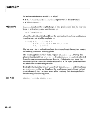
![learnwh
Purpose Widrow-Hoff weight/bias learning function
learnwh
Syntax [dW,LS] = learnwh(W,P,Z,N,A,T,E,gW,gA,D,LP,LS)
[db,LS] = learnwh(b,ones(1,Q),Z,N,A,T,E,gW,gA,D,LP,LS)
info = learnwh(code)
Description learnwh is the Widrow-Hoff weight/bias learning function, and is also known
as the delta or least mean squared (LMS) rule.
learnwh(W,P,Z,N,A,T,E,gW,gA,D,LP,LS) takes several inputs,
W - S x R weight matrix (or S x 1 bias vector).
P - R x Q input vectors (or ones(1,Q)).
Z - S x Q weighted input vectors.
N - S x Q net input vectors.
A - S x Q output vectors.
T - S x Q layer target vectors.
E - S x Q layer error vectors.
gW - S x R weight gradient with respect to performance.
gA - S x Q output gradient with respect to performance.
D - S x S neuron distances.
LP - Learning parameters, none, LP = [].
LS - Learning state, initially should be = [].
and returns,
dW - S x R weight (or bias) change matrix.
LS - New learning state.
Learning occurs according to learnwh's learning parameter shown here with
its default value.
LP.lr - 0.01 - Learning rate.
learnwh(code) returns useful information for each code string:
'pnames' - Names of learning parameters.
'pdefaults' - Default learning parameters.
'needg' - Returns 1 if this function uses gW or gA.
13-103](https://image.slidesharecdn.com/nnet-090922002848-phpapp01/85/Neural-Network-Toolbox-MATLAB-505-320.jpg)
![learnwh
Examples Here we define a random input P and error E to a layer with a 2-element input
and 3 neurons. We also define the learning rate LR learning parameter.
p = rand(2,1);
e = rand(3,1);
lp.lr = 0.5;
Since learnwh only needs these values to calculate a weight change (see
algorithm below), we will use them to do so.
dW = learnwh([],p,[],[],[],[],e,[],[],[],lp,[])
Network Use You can create a standard network that uses learnwh with newlin.
To prepare the weights and the bias of layer i of a custom network to learn with
learnwh:
1 Set net.trainFcn to 'trainwb'. net.trainParam will automatically become
trainwb's default parameters.
2 Set net.adaptFcn to 'adaptwb'. net.adaptParam will automatically become
trainwb's default parameters.
3 Set each net.inputWeights{i,j}.learnFcn to 'learnwh'. Set each
net.layerWeights{i,j}.learnFcn to 'learnwh'. Set
net.biases{i}.learnFcn to 'learnwh'.
Each weight and bias learning parameter property will automatically be set to
learnwh's default parameters.
To train the network (or enable it to adapt):
1 Set net.trainParam (net.adaptParam) properties to desired values.
2 Call train(adapt).
See newlin for adaption and training examples.
Algorithm learnwh calculates the weight change dW for a given neuron from the neuron's
input P and error E, and the weight (or bias) learning rate LR, according to the
Widrow-Hoff learning rule:
dw = lr*e*pn'
13-104](https://image.slidesharecdn.com/nnet-090922002848-phpapp01/85/Neural-Network-Toolbox-MATLAB-506-320.jpg)
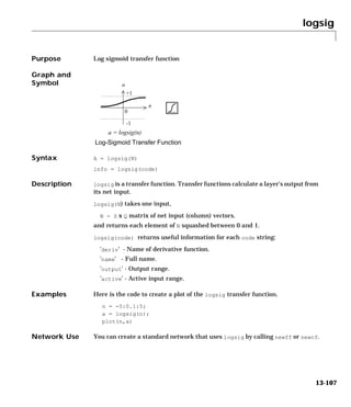

![mae
Purpose Mean absolute error performance function
mae
Syntax perf = mae(e,x,pp)
perf = mae(e,net,pp)
info = mae(code)
Description mae is a network performance function.
mae(E,X,PP) takes from one to three arguments,
E - Matrix or cell array of error vector(s).
X - Vector of all weight and bias values (ignored).
PP - Performance parameters (ignored).
and returns the mean absolute error.
The errors E can be given in cell array form,
E - Nt x TS cell array, each element E{i,ts} is a Vi x Q matrix or[].
or as a matrix,
E - (sum of Vi) x Q matrix
where
Nt = net.numTargets
TS = Number of time steps
Q = Batch size
Vi = net.targets{i}.size
mae(E,net,PP) can take an alternate argument to X,
net - Neural network from which X can be obtained (ignored).
mae(code) returns useful information for each code string:
'deriv' - Name of derivative function.
'name' - Full name.
'pnames' - Names of training parameters.
'pdefaults' - Default training parameters.
13-109](https://image.slidesharecdn.com/nnet-090922002848-phpapp01/85/Neural-Network-Toolbox-MATLAB-511-320.jpg)
![mae
Examples Here a perceptron is created with a 1-element input ranging from -10 to 10, and
one neuron.
net = newp([-10 10],1);
Here the network is given a batch of inputs P. The error is calculated by
subtracting the output A from target T. Then the mean absolute error is
calculated.
p = [-10 -5 0 5 10];
t = [0 0 1 1 1];
y = sim(net,p)
e = t-y
perf = mae(e)
Note that mae can be called with only one argument because the other
arguments are ignored. mae supports those arguments to conform to the
standard performance function argument list.
Network Use You can create a standard network that uses mae with newp.
To prepare a custom network to be trained with mae, set net.performFcn to
'mae'. This will automatically set net.performParam to the empty matrix [], as
mae has no performance parameters.
In either case, calling train or adapt will result in mae being used to calculate
performance.
See newp for examples.
See Also mse, msereg, dmae
13-110](https://image.slidesharecdn.com/nnet-090922002848-phpapp01/85/Neural-Network-Toolbox-MATLAB-512-320.jpg)
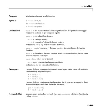

![mat2cell
Purpose Break matrix up into a cell array of matrices
mat2cell
Syntax mat2cell(M,R,C);
Description mat2cell(M,R,C) takes three arguments,
M - row x col matrix.
R - Vector of row sizes (should sum to row).
C - Vector of col sizes (should sum to col).
and returns a cell array of matrices, found using R and C.
Examples M = [1 2 3 4; 5 6 7 8; 9 10 11 12];
C = mat2cell(M,[1 2],[2 2])
See Also cell2mat
13-113](https://image.slidesharecdn.com/nnet-090922002848-phpapp01/85/Neural-Network-Toolbox-MATLAB-515-320.jpg)
![maxlinlr
Purpose Maximum learning rate for a linear layer
maxlinlr
Syntax lr = maxlinlr(P)
lr = maxlinlr(P,'bias')
Description maxlinlr is used to calculate learning rates for newlin.
maxlinlr(P) takes one argument,
P - R x Q matrix of input vectors.
and returns the maximum learning rate for a linear layer without a bias that
is to be trained only on the vectors in P.
maxlinlr(P,'bias') returns the maximum learning rate for a linear layer
with a bias.
Examples Here we define a batch of 4 2-element input vectors and find the maximum
learning rate for a linear layer with a bias.
P = [1 2 -4 7; 0.1 3 10 6];
lr = maxlinlr(P,'bias')
See Also linnet, newlin, newlind
13-114](https://image.slidesharecdn.com/nnet-090922002848-phpapp01/85/Neural-Network-Toolbox-MATLAB-516-320.jpg)
![midpoint
Purpose Midpoint weight initialization function
midpoint
Syntax W = midpoint(S,PR)
Description midpoint is a weight initialization function that sets weight (row) vectors to
the center of the input ranges.
midpoint(S,PR) takes two arguments,
S - Number of rows (neurons).
PR - R x 2 matrix of input value ranges = [Pmin Pmax].
and returns an S x R matrix with rows set to (Pmin+Pmax)'/2.
Examples Here initial weight values are calculated for a 5 neuron layer with input
elements ranging over [0 1] and [-2 2].
W = midpoint(5,[0 1; -2 2])
Network Use You can create a standard network that uses midpoint to initialize weights by
calling newc.
To prepare the weights and the bias of layer i of a custom network to initialize
with midpoint:
1 Set net.initFcn to 'initlay'. (net.initParam will automatically become
initlay's default parameters.)
2 Set net.layers{i}.initFcn to 'initwb'.
3 Set each net.inputWeights{i,j}.initFcn to 'midpoint'. Set each
net.layerWeights{i,j}.initFcn to 'midpoint';
To initialize the network call init.
See Also initwb, initlay, init
13-115](https://image.slidesharecdn.com/nnet-090922002848-phpapp01/85/Neural-Network-Toolbox-MATLAB-517-320.jpg)
![minmax
Purpose Ranges of matrix rows
minmax
Syntax pr = minmax(P)
Description minmax(P) takes one argument,
PR - R x Q matrix.
and returns the R x 2 matrix PR of minimum and maximum values for each row
of M.
Examples p = [0 1 2; -1 -2 -0.5]
pr = minmax(p)
13-116](https://image.slidesharecdn.com/nnet-090922002848-phpapp01/85/Neural-Network-Toolbox-MATLAB-518-320.jpg)
![mse
Purpose Mean squared error performance function
mse
Syntax perf = mse(e,x,pp)
perf = mse(e,net,pp)
info = mse(code)
Description mse is a network performance function. It measures the network’s performance
according to the mean of squared errors.
mse(E,X,PP) takes from one to three arguments,
E - Matrix or cell array of error vector(s).
X - Vector of all weight and bias values (ignored).
PP - Performance parameters (ignored).
and returns the mean squared error.
mse(E,net,PP) can take an alternate argument to X,
net - Neural network from which X can be obtained (ignored).
mse(code) returns useful information for each code string:
'deriv' - Name of derivative function.
'name' - Full name.
'pnames' - Names of training parameters.
'pdefaults' - Default training parameters.
Examples Here a two layer feed-forward network is created with a 1-element input
ranging from -10 to 10, four hidden tansig neurons, and one purelin output
neuron.
net = newff([-10 10],[4 1],{'tansig','purelin'});
13-117](https://image.slidesharecdn.com/nnet-090922002848-phpapp01/85/Neural-Network-Toolbox-MATLAB-519-320.jpg)
![mse
Here the network is given a batch of inputs P. The error is calculated by
subtracting the output A from target T. Then the mean squared error is
calculated.
p = [-10 -5 0 5 10];
t = [0 0 1 1 1];
y = sim(net,p)
e = t-y
perf = mse(e)
Note that mse can be called with only one argument because the other
arguments are ignored. mse supports those ignored arguments to conform to
the standard performance function argument list.
Network Use You can create a standard network that uses mse with newff, newcf, or newelm.
To prepare a custom network to be trained with mse, set net.performFcn to
'mse'. This will automatically set net.performParam to the empty matrix [], as
mse has no performance parameters.
In either case, calling train or adapt will result in mse being used to calculate
performance.
See newff or newcf for examples.
See Also msereg, mae, dmse
13-118](https://image.slidesharecdn.com/nnet-090922002848-phpapp01/85/Neural-Network-Toolbox-MATLAB-520-320.jpg)
![msereg
Purpose Mean squared error w/reg performance function
msereg
Syntax perf = mse(e,x,pp)
perf = mse(e,net,pp)
info = mse(code)
Description msereg is a network performance function. It measures network performance
as the weight sum of two factors: the mean squared error and the mean
squared weight and bias values.
msereg(E,X,PP) takes from three arguments,
E - Matrix or cell array of error vector(s).
X - Vector of all weight and bias values.
PP - Performance parameter.
where PP defines one performance parameters,
PP.ratio - Relative importance of errors vs. weight and bias values.
and returns the sum of mean squared errors (times PP.ratio) with the mean
squared weight and bias values (times 1-PP.ratio).
The errors E can be given in cell array form,
E - Nt x TS cell array, each element E{i,ts} is an Vi x Q matrix or [].
or as a matrix,
E - (sum of Vi) x Q matrix
where
Nt = net.numTargets
TS = Number of time steps
Q = Batch size
Vi = net.targets{i}.size
mse(E,net) takes an alternate argument to X and PP,
net - Neural network from which X and PP can be obtained.
13-119](https://image.slidesharecdn.com/nnet-090922002848-phpapp01/85/Neural-Network-Toolbox-MATLAB-521-320.jpg)
![msereg
mse(code) returns useful information for each code string:
'deriv' - Name of derivative function.
'name' - Full name.
'pnames' - Names of training parameters.
'pdefaults' - Default training parameters.
Examples Here a two layer feed-forward is created with a 1-element input ranging from
-2 to 2, four hidden tansig neurons, and one purelin output neuron.
net = newff([-2 2],[4 1]
{'tansig','purelin'},'trainlm','learngdm','msereg');
Here the network is given a batch of inputs P. The error is calculated by
subtracting the output A from target T. Then the mean squared error is
calculated using a ratio of 20/(20+1). (Errors are 20 times as important as
weight and bias values).
p = [-2 -1 0 1 2];
t = [0 1 1 1 0];
y = sim(net,p)
e = t-y
net.performParam.ratio = 20/(20+1);
perf = msereg(e,net)
Network Use You can create a standard network that uses msereg with newff, newcf, or
newelm.
To prepare a custom network to be trained with msereg, set net.performFcn
to 'msereg'. This will automatically set net.performParam to msereg's default
performance parameters.
In either case, calling train or adapt will result in msereg being used to
calculate performance.
See newff or newcf for examples.
See Also mse, mae, dmsereg
13-120](https://image.slidesharecdn.com/nnet-090922002848-phpapp01/85/Neural-Network-Toolbox-MATLAB-522-320.jpg)
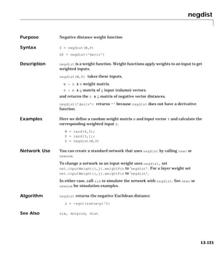
![netprod
Purpose Product net input function
netprod
Syntax N = netprod(Z1,Z2,...)
df = netprod('deriv')
Description netprod is a net input function. Net input functions calculate a layer's net
input by combining its weighted inputs and biases.
netprod(Z1,Z2,...,Zn)takes,
Zi - S x Q matrices.
and returns an element-wise sum of Zi's.
netprod('deriv') returns netprod's derivative function.
Examples Here netprod combines two sets of weighted input vectors (which we have
defined ourselves).
z1 = [1 2 4;3 4 1];
z2 = [-1 2 2; -5 -6 1];
n = netprod(z1,z2)
Here netprod combines the same weighted inputs with a bias vector. Because
Z1 and Z2 each contain three concurrent vectors, three concurrent copies of B
must be created with concur so that all sizes match up.
b = [0; -1];
n = netprod(z1,z2,concur(b,3))
Network Use You can create a standard network that uses netprod by calling newpnn or
newgrnn.
To change a network so that a layer uses netprod, set
net.layers{i}.netInputFcn to 'netprod'.
In either case, call sim to simulate the network with netprod. See newpnn or
newgrnn for simulation examples.
See Also sim, dnetprod, netsum, concur.
13-122](https://image.slidesharecdn.com/nnet-090922002848-phpapp01/85/Neural-Network-Toolbox-MATLAB-524-320.jpg)
![netsum
Purpose Sum net input function
netsum
Syntax N = netsum(Z1,Z2,...)
df = netsum('deriv')
Description netsum is a net input function. Net input functions calculate a layer's net input
by combining its weighted inputs and biases.
netsum(Z1,Z2,...,Zn) takes any number of inputs,
Zi - S x Q matrices,
and returns N, the element-wise sum of Zi's.
netsum('deriv') returns netsum's derivative function.
Examples Here netsum combines two sets of weighted input vectors (which we have
defined ourselves).
z1 = [1 2 4;3 4 1];
z2 = [-1 2 2; -5 -6 1];
n = netsum(z1,z2)
Here netsum combines the same weighted inputs with a bias vector. Because
Z1 and Z2 each contain three concurrent vectors, three concurrent copies of B
must be created with concur so that all sizes match up.
b = [0; -1];
n = netsum(z1,z2,concur(b,3))
Network Use You can create a standard network that uses netsum by calling newp or newlin.
To change a network so a layer uses netsum, set net.layers{i}.netInputFcn
to 'netsum'.
In either case, call sim to simulate the network with netsum. See newp or
newlin for simulation examples.
See Also sim, dnetprod, netprod, concur
13-123](https://image.slidesharecdn.com/nnet-090922002848-phpapp01/85/Neural-Network-Toolbox-MATLAB-525-320.jpg)

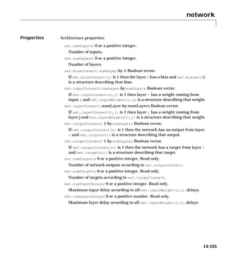
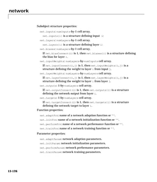
![network
Weight and bias value properties:
net.IW: numLayers-by-numInputs cell array of input weight values.
net.LW: numLayers-by-numLayers cell array of layer weight values.
net.b: numLayers-by-1 cell array of bias values.
Other properties:
net.userdata: structure you can use to store useful values.
Examples Here is the code to create a network without any inputs and layers, and then
set its number of inputs and layer to 1 and 2 respectively.
net = network
net.numInputs = 1
net.numLayers = 2
Here is the code to create the same network with one line of code.
net = network(1,2)
Here is the code to create a 1 input, 2 layer, feed-forward network. Only the
first layer will have a bias. An input weight will connect to layer 1 from input
1. A layer weight will connect to layer 2 from layer 1. Layer 2 will be a network
output, and have a target.
net = network(1,2,[1;0],[1; 0],[0 0; 1 0],[0 1],[0 1])
We can then see the properties of subobjects as follows:
net.inputs{1}
net.layers{1}, net.layers{2}
net.biases{1}
net.inputWeights{1,1}, net.layerWeights{2,1}
net.outputs{2}
net.targets{2}
We can get the weight matrices and bias vector as follows:
net.iw.{1,1}, net.iw{2,1}, net.b{1}
13-127](https://image.slidesharecdn.com/nnet-090922002848-phpapp01/85/Neural-Network-Toolbox-MATLAB-529-320.jpg)
![network
We can alter the properties of any of these subobjects. Here we change the
transfer functions of both layers:
net.layers{1}.transferFcn = 'tansig';
net.layers{2}.transferFcn = 'logsig';
Here we change the number of elements in input 1 to 2, by setting each
element’s range:
net.inputs{1}.range = [0 1; -1 1];
Next we can simulate the network for a 2-element input vector:
p = [0.5; -0.1];
y = sim(net,p)
See Also sim
13-128](https://image.slidesharecdn.com/nnet-090922002848-phpapp01/85/Neural-Network-Toolbox-MATLAB-530-320.jpg)
![newc
Purpose Create a competitive layer
newc
Syntax net = newc(PR,S,KLR,CLR)
Description Competitive layers are used to solve classification problems.
net = newc(PR,S,KLR,CLR) takes these inputs,
PR - R x 2 matrix of min and max values for R input elements.
S - Number of neurons.
KLR - Kohonen learning rate, default = 0.01.
CLR - Conscience learning rate, default = 0.001.
and returns a new competitive layer.
Properties Competitive layers consist of a single layer with the negdist weight function,
netsum net input function, and the compet transfer function.
The layer has a weight from the input, and a bias.
Weights and biases are initialized with midpoint and initcon.
Adaption and training are done with adaptwb and trainwb1, which both update
weight and bias values with the learnk and learncon learning functions.
Examples Here is a set of four two-element vectors P.
P = [.1 .8 .1 .9; .2 .9 .1 .8];
To competitive layer can be used to divide these inputs into two classes. First
a two neuron layer is created with two input elements ranging from 0 to 1, then
it is trained.
net = newc([0 1; 0 1],2);
net = train(net,P);
The resulting network can then be simulated and its output vectors converted
to class indices.
Y = sim(net,P)
Yc = vec2ind(Y)
See Also sim, init, adapt, train, adaptwb, trainwb1
13-129](https://image.slidesharecdn.com/nnet-090922002848-phpapp01/85/Neural-Network-Toolbox-MATLAB-531-320.jpg)
![newcf
Purpose Trainable cascade-forward backpropagation network
newcf
Syntax net = newcf(Pr,[S1 S2...SNl],{TF1 TF2...TFNl},BTF,BLF,PF)
Description newcf(PR,[S1 S2...SNl],{TF1 TF2...TFNl},BTF,BLF,PF) takes,
PR - R x 2 matrix of min and max values for R input elements.
Si - Size of ith layer, for Nl layers.
TFi - Transfer function of ith layer, default = 'tansig'.
BTF - Backprop network training function, default = 'traingd'.
BLF - Backprop weight/bias learning function, default = 'learngdm'.
PF - Performance function, default = 'mse'.
and returns an N layer cascade-forward backprop network.
The transfer functions TFi can be any differentiable transfer function such as
tansig, logsig, or purelin.
The training function BTF can be any of the backprop training functions such
as trainlm, trainbfg, trainrp, traingd, etc.
WARNING: trainlm is the default training function because it is very fast, but
it requires a lot of memory to run. If you get an out-of-memory error when
training try doing one of these:
1 Slow trainlm training, but reduce memory requirements by setting
net.trainParam.mem_reduc to 2 or more. (See help trainlm.)
2 Use trainbfg, which is slower but more memory-efficient than trainlm.
3 Use trainrp which is slower but more memory-efficient than trainbfg.
The learning function BLF can be either of the backpropagation learning
functions such as learngd, or learngdm.
The performance function can be any of the differentiable performance
functions such as mse or msereg.
Examples Here is a problem consisting of inputs P and targets T that we would like to
solve with a network.
P = [0 1 2 3 4 5 6 7 8 9 10];
T = [0 1 2 3 4 3 2 1 2 3 4];
13-130](https://image.slidesharecdn.com/nnet-090922002848-phpapp01/85/Neural-Network-Toolbox-MATLAB-532-320.jpg)
![newcf
Here a two-layer cascade-forward network is created. The network's input
ranges from [0 to 10]. The first layer has five tansig neurons, the second layer
has one purelin neuron. The trainlm network training function is to be used.
net = newcf([0 10],[5 1],{'tansig' 'purelin'});
Here the network is simulated and its output plotted against the targets.
Y = sim(net,P);
plot(P,T,P,Y,'o')
Here the network is trained for 50 epochs. Again the network's output is
plotted.
net.trainParam.epochs = 50;
net = train(net,P,T);
Y = sim(net,P);
plot(P,T,P,Y,'o')
Algorithm Cascade-forward networks consist of Nl layers using the dotprod weight
function, netsum net input function, and the specified transfer functions.
The first layer has weights coming from the input. Each subsequent layer has
weights coming from the input and all previous layers. All layers have biases.
The last layer is the network output.
Each layer's weights and biases are initialized with initnw.
Adaption is done with adaptwb which updates weights with the specified
learning function. Training is done with the specified training function.
Performance is measured according to the specified performance function.
See Also newff, newelm, sim, init, adapt, train
13-131](https://image.slidesharecdn.com/nnet-090922002848-phpapp01/85/Neural-Network-Toolbox-MATLAB-533-320.jpg)
![newelm
Purpose Create an Elman backpropagation network
newelm
Syntax net = newelm(PR,[S1 S2...SNl],{TF1 TF2...TFNl},BTF,BLF,PF)
Description newelm(PR,[S1 S2...SNl],{TF1 TF2...TFNl},BTF,BLF,PF) takes several
arguments,
PR - R x 2 matrix of min and max values for R input elements.
Si - Size of ith layer, for Nl layers.
TFi - Transfer function of ith layer, default = 'tansig'.
BTF - Backprop network training function, default = 'traingdx'.
BLF - Backprop weight/bias learning function, default = 'learngdm'.
PF - Performance function, default = 'mse'.
and returns an Elman network.
The training function BTF can be any of the backprop training functions such
as trainlm, trainbfg, trainrp, traingd, etc.
WARNING: trainlm is the default training function because it is very fast, but
it requires a lot of memory to run. If you get an "out-of-memory" error when
training try doing one of these:
1 Slow trainlm training, but reduce memory requirements by setting
net.trainParam.mem_reduc to 2 or more. (See help trainlm.)
2 Use trainbfg, which is slower but more memory-efficient than trainlm.
3 Use trainrp which is slower but more memory-efficient than trainbfg.
The learning function BLF can be either of the backpropagation learning
functions such as learngd, or learngdm.
The performance function can be any of the differentiable performance
functions such as mse or msereg.
Examples Here is a series of Boolean inputs P, and another sequence T, which is 1
wherever P has had two 1's in a row.
P = round(rand(1,20));
T = [0 (P(1:end-1)+P(2:end) == 2)];
13-132](https://image.slidesharecdn.com/nnet-090922002848-phpapp01/85/Neural-Network-Toolbox-MATLAB-534-320.jpg)
![newelm
We would like the network to recognize whenever two 1's occur in a row. First
we arrange these values as sequences.
Pseq = con2seq(P);
Tseq = con2seq(T);
Next we create an Elman network whose input varies from 0 to 1, and has five
hidden neurons and 1 output.
net = newelm([0 1],[10 1],{'tansig','logsig'});
Then we train the network with a mean squared error goal of 0.1, and simulate
it.
net = train(net,Pseq,Tseq);
Y = sim(net,Pseq)
Algorithm Elman networks consist of Nl layers using the dotprod weight function, netsum
net input function, and the specified transfer functions.
The first layer has weights coming from the input. Each subsequent layer has
a weight coming from the previous layer. All layers except the last have a
recurrent weight. All layers have biases. The last layer is the network output.
Each layer's weights and biases are initialized with initnw.
Adaption is done with adaptwb which updates weights with the specified
learning function. Training is done with the specified training function.
Performance is measured according to the specified performance function.
See Also newff, newcf, sim, init, adapt, train
13-133](https://image.slidesharecdn.com/nnet-090922002848-phpapp01/85/Neural-Network-Toolbox-MATLAB-535-320.jpg)
![newff
Purpose Create a feed-forward backpropagation network
newff
Syntax net = newff(PR,[S1 S2...SNl],{TF1 TF2...TFNl},BTF,BLF,PF)
Description newff(PR,[S1 S2...SNl],{TF1 TF2...TFNl},BTF,BLF,PF) takes,
PR - R x 2 matrix of min and max values for R input elements.
Si - Size of ith layer, for Nl layers.
TFi - Transfer function of ith layer, default = 'tansig'.
BTF - Backprop network training function, default = 'traingdx'.
BLF - Backprop weight/bias learning function, default = 'learngdm'.
PF - Performance function, default = 'mse'.
and returns an N layer feed-forward backprop network.
The transfer functions TFi can be any differentiable transfer function such as
tansig, logsig, or purelin.
The training function BTF can be any of the backprop training functions such
as trainlm, trainbfg, trainrp, traingd, etc.
WARNING: trainlm is the default training function because it is very fast, but
it requires a lot of memory to run. If you get an "out-of-memory" error when
training try doing one of these:
1 Slow trainlm training, but reduce memory requirements by setting
net.trainParam.mem_reduc to 2 or more. (See help trainlm.)
2 Use trainbfg, which is slower but more memory-efficient than trainlm.
3 Use trainrp which is slower but more memory-efficient than trainbfg.
The learning function BLF can be either of the backpropagation learning
functions such as learngd, or learngdm.
The performance function can be any of the differentiable performance
functions such as mse or msereg.
Examples Here is a problem consisting of inputs P and targets T that we would like to
solve with a network.
P = [0 1 2 3 4 5 6 7 8 9 10];
T = [0 1 2 3 4 3 2 1 2 3 4];
13-134](https://image.slidesharecdn.com/nnet-090922002848-phpapp01/85/Neural-Network-Toolbox-MATLAB-536-320.jpg)
![newff
Here a two-layer feed-forward network is created. The network's input ranges
from [0 to 10]. The first layer has five tansig neurons, the second layer has one
purelin neuron. The trainlm network training function is to be used.
net = newff([0 10],[5 1],{'tansig' 'purelin'});
Here the network is simulated and its output plotted against the targets.
Y = sim(net,P);
plot(P,T,P,Y,'o')
Here the network is trained for 50 epochs. Again the network's output is
plotted.
net.trainParam.epochs = 50;
net = train(net,P,T);
Y = sim(net,P);
plot(P,T,P,Y,'o')
Algorithm Feed-forward networks consist of Nl layers using the dotprod weight function,
netsum net input function, and the specified transfer functions.
The first layer has weights coming from the input. Each subsequent layer has
a weight coming from the previous layer. All layers have biases. The last layer
is the network output.
Each layer's weights and biases are initialized with initnw.
Adaption is done with adaptwb which updates weights with the specified
learning function. Training is done with the specified training function.
Performance is measured according to the specified performance function.
See Also newcf, newelm, sim, init, adapt, train
13-135](https://image.slidesharecdn.com/nnet-090922002848-phpapp01/85/Neural-Network-Toolbox-MATLAB-537-320.jpg)
![newfftd
Purpose Create a feed-forward input-delay backprop network
newfftd
Syntax net = newfftd(PR,ID,[S1 S2...SNl],{TF1 TF2...TFNl},BTF,BLF,PF)
Description newfftd(PR,ID,[S1 S2...SNl],{TF1 TF2...TFNl},BTF,BLF,PF) takes,
PR - R x 2 matrix of min and max values for R input elements.
ID - Input delay vector.
Si - Size of ith layer, for Nl layers.
TFi - Transfer function of ith layer, default = 'tansig'.
BTF - Backprop network training function, default = 'traingdx'.
BLF - Backprop weight/bias learning function, default = 'learngdm'.
PF - Performance function, default = 'mse'.
and returns an N layer feed-forward backprop network.
The transfer functions TFi can be any differentiable transfer function such as
tansig, logsig, or purelin.
The training function BTF can be any of the backprop training functions such
as trainlm, trainbfg, trainrp, traingd, etc.
WARNING: trainlm is the default training function because it is very fast, but
it requires a lot of memory to run. If you get an "out-of-memory" error when
training try doing one of these:
1 Slow trainlm training, but reduce memory requirements by setting
net.trainParam.mem_reduc to 2 or more. (See help trainlm.)
2 Use trainbfg, which is slower but more memory-efficient than trainlm.
3 Use trainrp which is slower but more memory-efficient than trainbfg.
The learning function BLF can be either of the backpropagation learning
functions such as learngd, or learngdm.
The performance function can be any of the differentiable performance
functions such as mse or msereg.
13-136](https://image.slidesharecdn.com/nnet-090922002848-phpapp01/85/Neural-Network-Toolbox-MATLAB-538-320.jpg)
![newfftd
Examples Here is a problem consisting of an input sequence P and target sequence T that
can be solved by a network with one delay.
P = {1 0 0 1 1 0 1 0 0 0 0 1 1 0 0 1};
T = {1 -1 0 1 0 -1 1 -1 0 0 0 1 0 -1 0 1};
Here a two-layer feed-forward network is created with input delays of 0 and 1.
The network's input ranges from [0 to 1]. The first layer has five tansig
neurons, the second layer has one purelin neuron. The trainlm network
training function is to be used.
net = newfftd([0 1],[0 1],[5 1],{'tansig' 'purelin'});
Here the network is simulated.
Y = sim(net,P)
Here the network is trained for 50 epochs. Again the network's output is
calculated.
net.trainParam.epochs = 50;
net = train(net,P,T);
Y = sim(net,P)
Algorithm Feed-forward networks consist of Nl layers using the dotprod weight function,
netsum net input function, and the specified transfer functions.
The first layer has weights coming from the input with the specified input
delays. Each subsequent layer has a weight coming from the previous layer. All
layers have biases. The last layer is the network output.
Each layer's weights and biases are initialized with initnw.
Adaption is done with adaptwb which updates weights with the specified
learning function. Training is done with the specified training function.
Performance is measured according to the specified performance function.
See Also newcf, newelm, sim, init, adapt, train
13-137](https://image.slidesharecdn.com/nnet-090922002848-phpapp01/85/Neural-Network-Toolbox-MATLAB-539-320.jpg)
![newgrnn
Purpose Design a generalized regression neural network
newgrnn
Syntax net = newgrnn(P,T,spread)
Description Generalized regression neural networks are a kind of radial basis network that
is often used for function approximation. grnn’s can be designed very quickly.
newgrnn(P,T,spread) takes three inputs,
P - R x Q matrix of Q input vectors.
T - S x Q matrix of Q target class vectors.
spread - Spread of radial basis functions, default = 1.0.
and returns a new generalized regression neural network.
The larger the spread, is the smoother the function approximation will be. To
fit data very closely, use a spread smaller than the typical distance between
input vectors. To fit the data more smoothly, use a larger spread.
Properties newgrnn creates a two layer network. The first layer has radbas neurons,
calculates weighted inputs with dist and net input with netprod. The second
layer has purelin neurons, calculates weighted input with normprod and net
inputs with netsum. Only the first layer has biases.
newgrnn sets the first layer weights to P', and the first layer biases are all set
to 0.8326/spread, resulting in radial basis functions that cross 0.5 at weighted
inputs of +/- spread. The second layer weights W2 are set to T.
Examples Here we design a radial basis network given inputs P and targets T.
P = [1 2 3];
T = [2.0 4.1 5.9];
net = newgrnn(P,T);
Here the network is simulated for a new input.
P = 1.5;
Y = sim(net,P)
See Also sim, newrb, newrbe, newpnn
References Wasserman, P.D., Advanced Methods in Neural Computing, New York: Van
Nostrand Reinhold, pp. 155-61, 1993.
13-138](https://image.slidesharecdn.com/nnet-090922002848-phpapp01/85/Neural-Network-Toolbox-MATLAB-540-320.jpg)
![newhop
Purpose Create a Hopfield recurrent network
newhop
Syntax net = newhop(T)
Description Hopfield networks are used for pattern recall.
newhop(T) takes one input argument,
T - R x Q matrix of Q target vectors. (Values must be +1 or -1.)
and returns a new Hopfield recurrent neural network with stable points at the
vectors in T.
Properties Hopfield networks consist of a single layer with the dotprod weight function,
netsum net input function, and the satlins transfer function.
The layer has a recurrent weight from itself and a bias.
Examples Here we create a Hopfield network with two three-element stable points T.
T = [-1 -1 1; 1 -1 1]';
net = newhop(T);
Below we check that the network is stable at these points by using them as
initial layer delay conditions. If the network is stable we would expect that the
outputs Y will be the same. (Since Hopfield networks have no inputs, the second
argument to sim is Q = 2 when using matrix notation).
Ai = T;
[Y,Pf,Af] = sim(net,2,[],Ai);
Y
To see if the network can correct a corrupted vector, run the following code
which simulates the Hopfield network for five timesteps. (Since Hopfield
networks have no inputs, the second argument to sim is {Q TS} = [1 5] when
using cell array notation.)
Ai = {[-0.9; -0.8; 0.7]};
[Y,Pf,Af] = sim(net,{1 5},{},Ai);
Y{1}
If you run the above code, Y{1} will equal T(:,1) if the network has managed
to convert the corrupted vector Ai to the nearest target vector.
13-139](https://image.slidesharecdn.com/nnet-090922002848-phpapp01/85/Neural-Network-Toolbox-MATLAB-541-320.jpg)

![newlin
Purpose Create a linear layer
newlin
Syntax net = newlin(PR,S,ID,LR)
new = newlin
Description Linear layers are often used as adaptive filters for signal processing and
prediction.
newlin(PR,S,ID,LR) takes these arguments,
PR - R x 2 matrix of min and max values for R input elements.
S - Number of elements in the output vector.
ID - Input delay vector, default = [0].
LR - Learning rate, default = 0.01.
and returns a new linear layer.
net = newlin(PR,S,0,P) takes an alternate argument,
P - Matrix of input vectors.
and returns a linear layer with the maximum stable learning rate for learning
with inputs P.
Call newlin without input arguments to define the network's attributes in a
dialog window.
Examples This code creates a single input (range of [-1 1] linear layer with one neuron,
input delays of 0 and 1, and a learning rate of 0.01. It is simulated for an input
sequence P1.
net = newlin([-1 1],1,[0 1],0.01);
P1 = {0 -1 1 1 0 -1 1 0 0 1};
Y = sim(net,P1)
Here targets T1 are defined and the layer adapts to them. (Since this is the first
call to adapt, the default input delay conditions are used.)
T1 = {0 -1 0 2 1 -1 0 1 0 1};
[net,Y,E,Pf] = adapt(net,P1,T1); Y
13-141](https://image.slidesharecdn.com/nnet-090922002848-phpapp01/85/Neural-Network-Toolbox-MATLAB-543-320.jpg)
![newlin
Here the linear layer continues to adapt for a new sequence using the previous
final conditions PF as initial conditions.
P2 = {1 0 -1 -1 1 1 1 0 -1};
T2 = {2 1 -1 -2 0 2 2 1 0};
[net,Y,E,Pf] = adapt(net,P2,T2); Y
Here we initialize the layer's weights and biases to new values.
net = init(net);
Here we train the newly initialized layer on the entire sequence for 200 epochs
to an error goal of 0.1.
P3 = [P1 P2];
T3 = [T1 T2];
net.trainParam.epochs = 200;
net.trainParam.goal = 0.1;
net = train(net,P3,T3);
Y = sim(net,[P1 P2])
Algorithm Linear layers consist of a single layer with the dotprod weight function, netsum
net input function, and purelin transfer function.
The layer has a weight from the input and a bias.
Weights and biases are initialized with initzero.
Adaption and training are done with adaptwb and trainwb, which both update
weight and bias values with learnwh. Performance is measured with mse.
See Also newlind, sim, init, adapt, train
13-142](https://image.slidesharecdn.com/nnet-090922002848-phpapp01/85/Neural-Network-Toolbox-MATLAB-544-320.jpg)
![newlind
Purpose Design a linear layer
newlind
Syntax net = newlind(P,T)
new = newlind
Description newlind(P,T) takes two input arguments,
P - R x Q matrix of Q input vectors.
T - S x Q matrix of Q target class vectors.
and returns a linear layer designed to output T (with minimum sum square
error) given input P.
Call newlind without input arguments to define the network's attributes in a
dialog window.
Examples We would like a linear layer that outputs T given P for the following definitions.
P = [1 2 3];
T = [2.0 4.1 5.9];
Here we use newlind to design such a network and check its response.
net = newlind(P,T);
Y = sim(net,P)
Algorithm newlind calculates weight W and bias B values for a linear layer from inputs P
and targets T by solving this linear equation in the least squares sense:
[W b] * [P; ones] = T
See Also sim, newlin
13-143](https://image.slidesharecdn.com/nnet-090922002848-phpapp01/85/Neural-Network-Toolbox-MATLAB-545-320.jpg)
![newlvq
Purpose Create a learning vector quantization network
newlvq
Syntax net = newlvq(PR,S1,PC,LR,LF)
Description LVQ networks are used to solve classification problems.
net = newlvq(PR,S1,PC,LR,LF) takes these inputs,
PR - R x 2 matrix of min and max values for R input elements.
S1 - Number of hidden neurons.
PC - S2 element vector of typical class percentages.
LR - Learning rate, default = 0.01.
LF - Learning function, default = 'learnlv2'.
returns a new LVQ network.
The learning function LF can be learnlv1 or learnlv2.
Properties newlvq creates a two layer network. The first layer uses the compet transfer
function, calculates weighted inputs with negdist, and net input with netsum.
The second layer has purelin neurons, calculates weighted input with dotprod
and net inputs with netsum. Neither layer has biases.
First layer weights are initialized with midpoint. The second layer weights are
set so that each output neuron i has unit weights coming to it from PC(i)
percent of the hidden neurons.
Adaption and training are done with adaptwb and trainwb1, which both update
the first layer weights with the specified learning functions.
Examples The input vectors P and target classes Tc below define a classification problem
to be solved by an LVQ network.
P = [-3 -2 -2 0 0 0 0 +2 +2 +3; ...
0 +1 -1 +2 +1 -1 -2 +1 -1 0];
Tc = [1 1 1 2 2 2 2 1 1 1];
13-144](https://image.slidesharecdn.com/nnet-090922002848-phpapp01/85/Neural-Network-Toolbox-MATLAB-546-320.jpg)
![newlvq
The target classes Tc are converted to target vectors T. Then, an LVQ network
is created (with inputs ranges obtained from P, 4 hidden neurons, and class
percentages of 0.6 and 0.4) and is trained.
T = ind2vec(Tc);
net = newlvq(minmax(P),4,[.6 .4]);
net = train(net,P,T);
The resulting network can be tested.
Y = sim(net,P)
Yc = vec2ind(Y)
See Also sim, init, adapt, train, adaptwb, trainwb1, learnlv1, learnlv2
13-145](https://image.slidesharecdn.com/nnet-090922002848-phpapp01/85/Neural-Network-Toolbox-MATLAB-547-320.jpg)
![newp
Purpose Create a perceptron
newp
Syntax net = newp(pr,s,tf,lf)
Description Perceptrons are used to solve simple (i.e. linearly separable) classification
problems.
net = newp(PR,S,TF,LF) takes these inputs,
PR - R x 2 matrix of min and max values for R input elements.
S - Number of neurons.
TF - Transfer function, default = 'hardlim'.
LF - Learning function, default = 'learnp'.
and returns a new perceptron.
The transfer function TF can be hardlim or hardlims. The learning function LF
can be learnp or learnpn.
Call newp without input arguments to define the network's attributes in a
dialog window.
Properties Perceptrons consist of a single layer with the dotprod weight function, the
netsum net input function, and the specified transfer function.
The layer has a weight from the input and a bias.
Weights and biases are initialized with initzero.
Adaption and training are done with adaptwb and trainwb, which both update
weight and bias values with the specified learning function. Performance is
measured with mae.
Examples This code creates a perceptron layer with one 2-element input (ranges [0 1] and
[-2 2]) and one neuron. (Supplying only two arguments to newp results in the
default perceptron learning function learnp being used.)
net = newp([0 1; -2 2],1);
Here we simulate the network to a sequence of inputs P.
P1 = {[0; 0] [0; 1] [1; 0] [1; 1]};
Y = sim(net,P1)
13-146](https://image.slidesharecdn.com/nnet-090922002848-phpapp01/85/Neural-Network-Toolbox-MATLAB-548-320.jpg)
![newp
Here we define a sequence of targets T (together P and T define the operation of
an AND gate), and then let the network adapt for 10 passes through the
sequence. We then simulate the updated network.
T1 = {0 0 0 1};
net.adaptParam.passes = 10;
net = adapt(net,P1,T1);
Y = sim(net,P1)
Now we define a new problem, an OR gate, with batch inputs P and targets T.
P2 = [0 0 1 1; 0 1 0 1];
T2 = [0 1 1 1];
Here we initialize the perceptron (resulting in new random weight and bias
values), simulate its output, train for a maximum of 20 epochs, and then
simulate it again.
net = init(net);
Y = sim(net,P2)
net.trainParam.epochs = 20;
net = train(net,P2,T2);
Y = sim(net,P2)
Notes Perceptrons can classify linearly separable classes in a finite amount of time.
If input vectors have a large variance in their lengths, the learnpn can be
faster than learnp.
See Also sim, init, adapt, train, hardlim, hardlims, learnp, learnpn
13-147](https://image.slidesharecdn.com/nnet-090922002848-phpapp01/85/Neural-Network-Toolbox-MATLAB-549-320.jpg)
![newpnn
Purpose Design a probabilistic neural network
newpnn
Syntax net = newpnn(P,T,spread)
Description Probabilistic neural networks are a kind of radial basis network suitable for
classification problems.
net = newpnn(P,T,spread)takes two or three arguments,
P - R x Q matrix of Q input vectors.
T - S x Q matrix of Q target class vectors.
spread - Spread of radial basis functions, default = 0.1.
and returns a new probabilistic neural network.
If spread is near zero the network will act as a nearest neighbor classifier. As
spread becomes larger the designed network will take into account several
nearby design vectors.
Examples Here a classification problem is defined with a set of inputs P and class indices
Tc.
P = [1 2 3 4 5 6 7];
Tc = [1 2 3 2 2 3 1];
Here the class indices are converted to target vectors, and a PNN is designed
and tested.
T = ind2vec(Tc)
net = newpnn(P,T);
Y = sim(net,P)
Yc = vec2ind(Y)
Algorithm newpnn creates a two layer network. The first layer has radbas neurons, and
calculates its weighted inputs with dist, and its net input with netprod. The
second layer has compet neurons, and calculates its weighted input with
dotprod and its net inputs with netsum. Only the first layer has biases.
newpnn sets the first layer weights to P', and the first layer biases are all set to
0.8326/spread resulting in radial basis functions that cross 0.5 at weighted
inputs of +/- spread. The second layer weights W2 are set to T.
13-148](https://image.slidesharecdn.com/nnet-090922002848-phpapp01/85/Neural-Network-Toolbox-MATLAB-550-320.jpg)
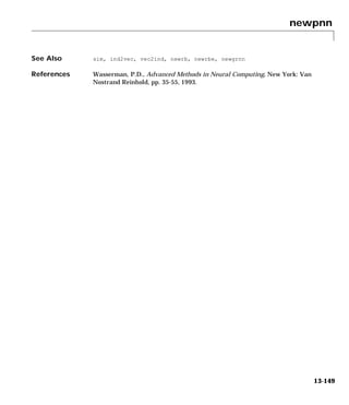
![newrb
Purpose Design a radial basis network
newrb
Syntax net = newrb(P,T,goal,spread)
Description Radial basis networks can be used to approximate functions. newrb adds
neurons to the hidden layer of a radial basis network until it meets the
specified mean squared error goal.
newrb(P,T,goal,spread) takes two to four arguments,
P - R x Q matrix of Q input vectors.
T - S x Q matrix of Q target class vectors.
goal - Mean squared error goal, default = 0.0.
spread - Spread of radial basis functions, default = 1.0.
and returns a new radial basis network.
The larger that spread is, the smoother the function approximation will be. Too
large a spread means a lot of neurons will be required to fit a fast changing
function. Too small a spread means many neurons will be required to fit a
smooth function, and the network may not generalize well. Call newrb with
different spreads to find the best value for a given problem.
Examples Here we design a radial basis network given inputs P and targets T.
P = [1 2 3];
T = [2.0 4.1 5.9];
net = newrb(P,T);
Here the network is simulated for a new input.
P = 1.5;
Y = sim(net,P)
Algorithm newrb creates a two layer network. The first layer has radbas neurons, and
calculates its weighted inputs with dist, and its net input with netprod. The
second layer has purelin neurons, and calculates its weighted input with
dotprod and its net inputs with netsum. Both layers have biases.
13-150](https://image.slidesharecdn.com/nnet-090922002848-phpapp01/85/Neural-Network-Toolbox-MATLAB-552-320.jpg)
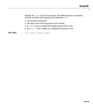
![newrbe
Purpose Design an exact radial basis network
newrbe
Syntax net = newrbe(P,T,spread)
Description Radial basis networks can be used to approximate functions. newrbe very
quickly designs a radial basis network with zero error on the design vectors.
newrbe(P,T,spread) takes two or three arguments,
P - R x Q matrix of Q input vectors.
T - S x Q matrix of Q target class vectors.
spread - Spread of radial basis functions, default = 1.0.
and returns a new exact radial basis network.
The larger the spread is, the smoother the function approximation will be. Too
large a spread can cause numerical problems.
Examples Here we design a radial basis network given inputs P and targets T.
P = [1 2 3];
T = [2.0 4.1 5.9];
net = newrbe(P,T);
Here the network is simulated for a new input.
P = 1.5;
Y = sim(net,P)
Algorithm newrbe creates a two layer network. The first layer has radbas neurons, and
calculates its weighted inputs with dist, and its net input with netprod. The
second layer has purelin neurons, and calculates its weighted input with
dotprod and its net inputs with netsum. Both layers have biases.
newrbe sets the first layer weights to P', and the first layer biases are all set to
0.8326/spread, resulting in radial basis functions that cross 0.5 at weighted
inputs of +/- spread.
The second layer weights IW{2,1} and biases b{2} are found by simulating the
first layer outputs A{1}, and then solving the following linear expression:
[W{2,1} b{2}] * [A{1}; ones] = T
See Also sim, newrb, newgrnn, newpnn
13-152](https://image.slidesharecdn.com/nnet-090922002848-phpapp01/85/Neural-Network-Toolbox-MATLAB-554-320.jpg)
![newsom
Purpose Create a self-organizing map
newsom
Syntax net = newsom(PR,[d1,d2,...],tfcn,dfcn,olr,osteps,tlr,tnd)
Description Competitive layers are used to solve classification problems.
net = newsom (PR,[D1,D2,...],TFCN,DFCN,OLR,OSTEPS,TLR,TND) takes,
PR - R x 2 matrix of min and max values for R input elements.
I - Size of ith layer dimension, defaults = [5 8].
TFCN - Topology function, default ='hextop'.
DFCN - Distance function, default ='linkdist'.
OLR - Ordering phase learning rate, default = 0.9.
OSTEPS - Ordering phase steps, default = 1000.
TLR - Tuning phase learning rate, default = 0.02;
TND - Tuning phase neighborhood distance, default = 1.
and returns a new self-organizing map.
The topology function TFCN can be hextop, gridtop, or randtop. The distance
function can be linkdist, dist, or mandist.
Properties Simms consist of a single layer with the negdist weight function, netsum net
input function, and the compet transfer function.
The layer has a weight from the input, but no bias. The weight is initialized
with midpoint.
Adaption and training are done with adaptwb and trainwb1, which both update
the weight with learnsom.
Examples The input vectors defined below are distributed over an 2-dimension input
space varying over [0 2] and [0 1]. This data will be used to train a SOM with
dimensions [3 5].
P = [rand(1,400)*2; rand(1,400)];
net = newsom([0 2; 0 1],[3 5]);
plotsom(net.layers{1}.positions)
13-153](https://image.slidesharecdn.com/nnet-090922002848-phpapp01/85/Neural-Network-Toolbox-MATLAB-555-320.jpg)
![nncopy
Purpose Copy matrix or cell array
nncopy
Syntax nncopy(x,m,n)
Description nncopy(X,M,N) takes two arguments,
X - R x C matrix (or cell array).
M - Number of vertical copies.
N - Number of horizontal copies.
and returns a new (R*M) x (C*N) matrix (or cell array).
Examples x1 = [1 2 3; 4 5 6];
y1 = nncopy(x1,3,2)
x2 = {[1 2]; [3; 4; 5]}
y2 = nncopy(x2,2,3)
13-155](https://image.slidesharecdn.com/nnet-090922002848-phpapp01/85/Neural-Network-Toolbox-MATLAB-557-320.jpg)
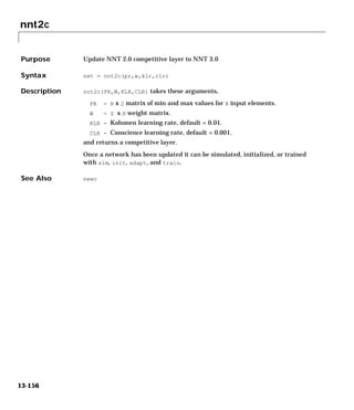
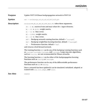
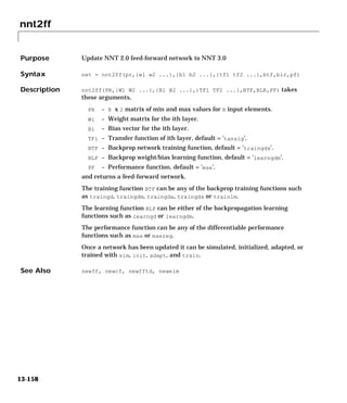

![nnt2som
Purpose Update NNT 2.0 self-organizing map to NNT 3.0
nnt2som
Syntax net = nnt2som(pr,[d1 d2 ...],w,olr,osteps,tlr,tnd)
Description nnt2som(PR,[D1,D2,...],W,OLR,OSTEPS,TLR,TND) takes these arguments,
PR - R x 2 matrix of min and max values for R input elements.
Di - Size of ith layer dimension.
W - S x R weight matrix.
OLR - Ordering phase learning rate, default = 0.9.
OSTEPS - Ordering phase steps, default = 1000.
TLR - Tuning phase learning rate, default = 0.02;
TND - Tuning phase neighborhood distance, default = 1.
and returns a self-organizing map.
nnt2som assumes that the self-organizing map has a grid topology (gridtop)
using link distances (linkdist). This corresponds with the nbman neighborhood
function in NNT 2.0.
The new network will only output 1 for the neuron with the greatest net input.
In NNT 2.0 the network would also output 0.5 for that neuron's neighbors.
Once a network has been updated it can be simulated, initialized, adapted, or
trained with sim, init, adapt, and train.
See Also newsom
13-164](https://image.slidesharecdn.com/nnet-090922002848-phpapp01/85/Neural-Network-Toolbox-MATLAB-566-320.jpg)
![normc
Purpose Normalize the columns of a matrix
normc
Syntax normc(M)
Description normc(M) normalizes the columns of M to a length of 1.
Examples m = [1 2; 3 4];
normc(m)
ans =
0.3162 0.4472
0.9487 0.8944
See Also normr
13-165](https://image.slidesharecdn.com/nnet-090922002848-phpapp01/85/Neural-Network-Toolbox-MATLAB-567-320.jpg)
![normr
Purpose Normalize the rows of a matrix
normr
Syntax normr(M)
Description normr(M) normalizes the columns of M to a length of 1.
Examples m = [1 2; 3 4];
normr(m)
ans =
0.4472 0.8944
0.6000 0.8000
See Also normc
13-167](https://image.slidesharecdn.com/nnet-090922002848-phpapp01/85/Neural-Network-Toolbox-MATLAB-569-320.jpg)
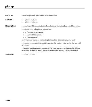
![plotes
Purpose Plot the error surface of a single input neuron
plotes
Syntax plotes(wv,bv,es,v)
Description plotes(WV,BV,ES,V) takes these arguments,
WV - 1 x N row vector of values of W.
BV - 1 x M row vector of values of B.
ES - M x N matrix of error vectors.
V - View, default = [-37.5, 30].
and plots the error surface with a contour underneath.
Calculate the error surface ES with errsurf.
Examples p = [3 2];
t = [0.4 0.8];
wv = -4:0.4:4; bv = wv;
ES = errsurf(p,t,wv,bv,'logsig');
plotes(wv,bv,ES,[60 30])
See Also errsurf
13-169](https://image.slidesharecdn.com/nnet-090922002848-phpapp01/85/Neural-Network-Toolbox-MATLAB-571-320.jpg)
![plotpc
Purpose Plot a classification line on a perceptron vector plot
plotpc
Syntax plotpc(W,b)
Description plotpc(W,B) takes these inputs,
W - S x R weight matrix (R must be 3 or less).
B - S x 1 bias vector.
and returns a handle to a plotted classification line.
plotpc(W,B,H) takes these inputs,
H - Handle to last plotted line.
and deletes the last line before plotting the new one.
This function does not change the current axis and is intended to be called after
plotpv.
Examples The code below defines and plots the inputs and targets for a perceptron:
p = [0 0 1 1; 0 1 0 1];
t = [0 0 0 1];
plotpv(p,t)
The following code creates a perceptron with inputs ranging over the values in
P, assigns values to its weights and biases, and plots the resulting classification
line.
net = newp(minmax(p),1);
net.iw{1,1} = [-1.2 -0.5];
net.b{1} = 1;
plotpc(net.iw{1,1},net.b{1})
See Also plotpv
13-170](https://image.slidesharecdn.com/nnet-090922002848-phpapp01/85/Neural-Network-Toolbox-MATLAB-572-320.jpg)
![plotperf
Purpose Plot network performance
plotperf
Syntax plotperf(tr,goal,name,epoch)
Description plotperf(TR,goal,name,epoch) takes these inputs,
TR - Training record returned by train.
goal - Performance goal, default = NaN.
name - Training function name, default = ''.
epoch - Number of epochs, default = length of training record.
and plots the training performance, and if available, the performance goal,
validation performance, and test performance.
Examples Here are 8 input values P and associated targets T, plus a like number of
validation inputs VV.P and targets VV.T.
P = 1:8; T = sin(P);
VV.P = P; VV.T = T+rand(1,8)*0.1;
The code below creates a network and trains it on this problem.
net = newff(minmax(P),[4 1],{'tansig','tansig'});
[net,tr] = train(net,P,T,[],[],VV);
During training plotperf was called to display the training record. You can
also call plotperf directly with the final training record TR, as shown below.
plotperf(tr)
13-171](https://image.slidesharecdn.com/nnet-090922002848-phpapp01/85/Neural-Network-Toolbox-MATLAB-573-320.jpg)
![plotpv
Purpose Plot perceptron input/target vectors
plotpv
Syntax plotpv(p,t)
Description plotpv(P,T) take these inputs,
P - R x Q matrix of input vectors (R must be 3 or less).
T - S x Q matrix of binary target vectors (S must be 3 or less).
and plots column vectors in P with markers based on T.
plotpv(P,T,V) takes an additional input,
V - Graph limits = [x_min x_max y_min y_max]
and plots the column vectors with limits set by V.
Examples The code below defines and plots the inputs and targets for a perceptron:
p = [0 0 1 1; 0 1 0 1];
t = [0 0 0 1];
plotpv(p,t)
The following code creates a perceptron with inputs ranging over the values in
P, assigns values to its weights and biases, and plots the resulting classification
line.
net = newp(minmax(p),1);
net.iw{1,1} = [-1.2 -0.5];
net.b{1} = 1;
plotpc(net.iw{1,1},net.b{1})
See Also plotpc
13-172](https://image.slidesharecdn.com/nnet-090922002848-phpapp01/85/Neural-Network-Toolbox-MATLAB-574-320.jpg)
![plotv
Purpose Plot vectors as lines from the origin
plotv
Syntax plotv(m,t)
Description plotv(M,T) takes two inputs,
M - R x Q matrix of Q column vectors with R elements.
T - (optional) the line plotting type, default = '-'.
and plots the column vectors of M.
R must be 2 or greater. If R is greater than two, only the first two rows of M are
used for the plot.
Examples plotv([-.4 0.7 .2; -0.5 .1 0.5],'-')
13-173](https://image.slidesharecdn.com/nnet-090922002848-phpapp01/85/Neural-Network-Toolbox-MATLAB-575-320.jpg)
![plotvec
Purpose Plot vectors with different colors
plotvec
Syntax plotvec(x,c,m)
Description plotvec(X,C,M) takes these inputs,
X - Matrix of (column) vectors.
C - Row vector of color coordinate.
M - Marker, default = '+'.
and plots each ith vector in X with a marker M and using the ith value in C as
the color coordinate.
plotvec(X) only takes a matrix X and plots each ith vector in X with marker
'+' using the index i as the color coordinate.
Examples x = [0 1 0.5 0.7; -1 2 0.5 0.1];
c = [1 2 3 4];
plotvec(x,c)
13-174](https://image.slidesharecdn.com/nnet-090922002848-phpapp01/85/Neural-Network-Toolbox-MATLAB-576-320.jpg)
![pnormc
Purpose Pseudo-normalize columns of a matrix
pnormc
Syntax pnormc(x,r)
Description pnormc(M,R) takes these arguments,
X - M x N matrix.
R - (optional) radius to normalize columns to, default = 1.
and returns X with an additional row of elements, which results in new column
vector lengths of R.
WARNING: For this function to work properly, the columns of X must
originally have vector lengths less than R.
Examples x = [0.1 0.6; 0.3 0.1];
y = pnormc(x)
See Also normc, normr
13-175](https://image.slidesharecdn.com/nnet-090922002848-phpapp01/85/Neural-Network-Toolbox-MATLAB-577-320.jpg)
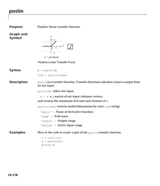

![postmnmx
Purpose Postprocess data which has been preprocessed by premnmx
postmnmx
Syntax [p,t] = postmnmx(pn,minp,maxp,tn,mint,maxt)
[p] = postmnmx(pn,minp,maxp)
Description postmnmx postprocesses the network training set which was preprocessed by
premnmx. It converts the data back into unnormalized units.
postmnmx takes these inputs,
PN - R x Q matrix of normalized input vectors.
minp- R x 1 vector containing minimums for each P.
maxp- R x 1 vector containing maximums for each P.
TN - S x Q matrix of normalized target vectors.
mint- S x 1 vector containing minimums for each T.
maxt- S x 1 vector containing maximums for each T.
and returns,
P - R x Q matrix of input (column) vectors.
T - R x Q matrix of target vectors.
Examples In this example we normalize a set of training data with premnmx, create and
train a network using the normalized data, simulate the network, unnormalize
the output of the network using postmnmx, and perform a linear regression
between the network outputs (unnormalized) and the targets to check the
quality of the network training.
p = [-0.92 0.73 -0.47 0.74 0.29; -0.08 0.86 -0.67 -0.52 0.93];
t = [-0.08 3.4 -0.82 0.69 3.1];
[pn,minp,maxp,tn,mint,maxt] = premnmx(p,t);
net = newff(minmax(pn),[5 1],{'tansig' 'purelin'},'trainlm');
net = train(net,pn,tn);
an = sim(net,pn);
[a] = postmnmx(an,mint,maxt);
[m,b,r] = postreg(a,t);
Algorithm p = 0.5(pn+1)*(maxp-minp) + minp;
See Also premnmx, prepca, poststd
13-178](https://image.slidesharecdn.com/nnet-090922002848-phpapp01/85/Neural-Network-Toolbox-MATLAB-580-320.jpg)
![postreg
Purpose Postprocess the trained network response with a linear regression
postreg
Syntax [m,b,r] = postreg(A,T)
Description postreg postprocesses the network training set by performing a linear
regression between each element of the network response and the
corresponding target.
postreg(A,T) takes these inputs,
A - 1 x Q array of network outputs. One element of the network output.
T - 1 x Q array of targets. One element of the target vector.
and returns,
M - Slope of the linear regression.
B - Y intercept of the linear regression.
R - Regression R-value. R=1 means perfect correlation.
Examples In this example we normalize a set of training data with prestd, perform a
principal component transformation on the normalized data, create and train
a network using the pca data, simulate the network, unnormalize the output
of the network using poststd, and perform a linear regression between the
network outputs (unnormalized) and the targets to check the quality of the
network training.
p = [-0.92 0.73 -0.47 0.74 0.29; -0.08 0.86 -0.67 -0.52 0.93];
t = [-0.08 3.4 -0.82 0.69 3.1];
[pn,meanp,stdp,tn,meant,stdt] = prestd(p,t);
[ptrans,transMat] = prepca(pn,0.02);
net = newff(minmax(ptrans),[5 1],{'tansig''purelin'},'trainlm');
net = train(net,ptrans,tn);
an = sim(net,ptrans);
a = poststd(an,meant,stdt);
[m,b,r] = postreg(a,t);
Algorithm Performs a linear regression between the network response and the target, and
then computes the correlation coefficient (R-value) between the network
response and the target.
See Also premnmx, prepca
13-179](https://image.slidesharecdn.com/nnet-090922002848-phpapp01/85/Neural-Network-Toolbox-MATLAB-581-320.jpg)
![poststd
Purpose Postprocess data which has been preprocessed by prestd
poststd
Syntax [p,t] = poststd(pn,meanp,stdp,tn,meant,stdt)
[p] = poststd(pn,meanp,stdp)
Description poststd postprocesses the network training set which was preprocessed by
prestd. It converts the data back into unnormalized units.
poststd takes these inputs,
PN - R x Q matrix of normalized input vectors.
meanp - R x 1 vector containing standard deviations for each P.
stdp - R x 1 vector containing standard deviations for each P.
TN - S x Q matrix of normalized target vectors.
meant - S x 1 vector containing standard deviations for each T.
stdt - S x 1 vector containing standard deviations for each T.
and returns,
P - R x Q matrix of input (column) vectors.
T - S x Q matrix of target vectors.
Examples In this example we normalize a set of training data with prestd, create and
train a network using the normalized data, simulate the network, unnormalize
the output of the network using poststd, and perform a linear regression
between the network outputs (unnormalized) and the targets to check the
quality of the network training.
p = [-0.92 0.73 -0.47 0.74 0.29; -0.08 0.86 -0.67 -0.52 0.93];
t = [-0.08 3.4 -0.82 0.69 3.1];
[pn,meanp,stdp,tn,meant,stdt] = prestd(p,t);
net = newff(minmax(pn),[5 1],{'tansig' 'purelin'},'trainlm');
net = train(net,pn,tn);
an = sim(net,pn);
a = poststd(an,meant,stdt);
[m,b,r] = postreg(a,t);
Algorithm p = stdp*pn + meanp;
See Also premnmx, prepca, postmnmx, prestd
13-180](https://image.slidesharecdn.com/nnet-090922002848-phpapp01/85/Neural-Network-Toolbox-MATLAB-582-320.jpg)
![premnmx
Purpose Preprocess data so that minimum is -1 and maximum is 1
premnmx
Syntax [pn,minp,maxp,tn,mint,maxt] = premnmx(p,t)
[pn,minp,maxp] = premnmx(p)
Description premnmx preprocesses the network training set by normalizing the inputs and
targets so that they fall in the interval [-1,1].
premnmx(P,T) takes these inputs,
P - R x Q matrix of input (column) vectors.
T - S x Q matrix of target vectors.
and returns,
PN - R x Q matrix of normalized input vectors.
minp- R x 1 vector containing minimums for each P.
maxp- R x 1 vector containing maximums for each P.
TN - S x Q matrix of normalized target vectors.
mint- S x 1 vector containing minimums for each T.
maxt- S x 1 vector containing maximums for each T.
Examples Here is the code to normalize a given data set so that the inputs and targets
will fall in the range [-1,1].
p = [-10 -7.5 -5 -2.5 0 2.5 5 7.5 10];
t = [0 7.07 -10 -7.07 0 7.07 10 7.07 0];
[pn,minp,maxp,tn,mint,maxt] = premnmx(p,t);
If you just want to normalize the input,
[pn,minp,maxp] = premnmx(p);
Algorithm pn = 2*(p-minp)/(maxp-minp) - 1;
See Also prestd, prepca, postmnmx
13-181](https://image.slidesharecdn.com/nnet-090922002848-phpapp01/85/Neural-Network-Toolbox-MATLAB-583-320.jpg)
![prepca
Purpose Principal component analysis
prepca
Syntax [ptrans,transMat] = prepca(P,min_frac)
Description prepca preprocesses the network input training set by applying a principal
component analysis. This analysis transforms the input data so that the
elements of the input vector set will be uncorrelated. In addition, the size of the
input vectors may be reduced by retaining only those components which
contribute more than a specified fraction (min_frac) of the total variation in
the data set.
prepca(p,min_frac) takes these inputs
P - R x Q matrix of centered input (column) vectors.
min_frac - Minimum fraction variance component to keep.
and returns
ptrans - Transformed data set.
transMat - Transformation matrix.
Examples Here is the code to perform a principal component analysis and retain only
those components which contribute more than 2 percent to the variance in the
data set. prestd is called first to create zero mean data, which are needed for
prepca.
p=[-1.5 -0.58 0.21 -0.96 -0.79; -2.2 -0.87 0.31 -1.4 -1.2];
[pn,meanp,stdp] = prestd(p);
[ptrans,transMat] = prepca(pn,0.02);
Since the second row of p is almost a multiple of the first row, this example will
produce a transformed data set which contains only one row.
Algorithm This routine uses singular value decomposition to compute the principal
components. The input vectors are multiplied by a matrix whose rows consist
of the eigenvectors of the input covariance matrix. This produces transformed
input vectors whose components are uncorrelated and ordered according to the
magnitude of their variance.
13-182](https://image.slidesharecdn.com/nnet-090922002848-phpapp01/85/Neural-Network-Toolbox-MATLAB-584-320.jpg)
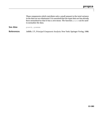
![prestd
Purpose Preprocess data so that its mean is 0 and the standard deviation is 1
prestd
Syntax [pn,meanp,stdp,tn,meant,stdt] = prestd(p,t)
[pn,meanp,stdp] = prestd(p)
Description prestd preprocesses the network training set by normalizing the inputs and
targets so that they have means of zero and standard deviations of 1.
prestd(p,t) takes these inputs,
p - R x Q matrix of input (column) vectors.
t - S x Q matrix of target vectors.
and returns,
pn - R x Q matrix of normalized input vectors.
meanp - R x 1 vector containing standard deviations for each P.
stdp - R x 1 vector containing standard deviations for each P.
tn - S x Q matrix of normalized target vectors.
meant - S x 1 vector containing standard deviations for each T.
stdt - S x 1 vector containing standard deviations for each T.
Examples Here is the code to normalize a given data set so that the inputs and targets
will have means of zero and standard deviations of 1.
p = [-0.92 0.73 -0.47 0.74 0.29; -0.08 0.86 -0.67 -0.52 0.93];
t = [-0.08 3.4 -0.82 0.69 3.1];
[pn,meanp,stdp,tn,meant,stdt] = prestd(p,t);
If you just want to normalize the input,
[pn,meanp,stdp] = prestd(p);
Algorithm pn = (p-meanp)/stdp;
See Also premnmx, prepca
13-184](https://image.slidesharecdn.com/nnet-090922002848-phpapp01/85/Neural-Network-Toolbox-MATLAB-586-320.jpg)
![quant
Purpose Discretize values as multiples of a quantity
quant
Syntax quant(X,q)
Description quant(X,q) takes two inputs,
X - Matrix, vector or scalar.
Q - Minimum value.
and returns values in X rounded to nearest multiple of Q.
Examples x = [1.333 4.756 -3.897];
y = quant(x,0.1)
13-186](https://image.slidesharecdn.com/nnet-090922002848-phpapp01/85/Neural-Network-Toolbox-MATLAB-588-320.jpg)
![randnc
Purpose Normalized column weight initialization function
randnc
Syntax W = randnc(S,PR)
W = randnc(S,R)
Description randnc is a weight initialization function.
randnc(S,P) takes two inputs,
S - Number of rows (neurons).
PR - R x 2 matrix of input value ranges = [Pmin Pmax].
and returns an S x R random matrix with normalized columns.
Can also be called as randnc(S,R).
Examples A random matrix of four normalized three-element columns is generated:
M = randnc(3,4)
M =
–0.6007 –0.4715 –0.2724 0.5596
–0.7628 –0.6967 –0.9172 0.7819
–0.2395 0.5406 –0.2907 0.2747
See Also randnr
13-188](https://image.slidesharecdn.com/nnet-090922002848-phpapp01/85/Neural-Network-Toolbox-MATLAB-590-320.jpg)
![randnr
Purpose Normalized row weight initialization function
randnr
Syntax W = randnr(S,PR)
W = randnr(S,R)
Description randnr is a weight initialization function.
randnr(S,P) takes two inputs,
S - Number of rows (neurons).
PR - R x 2 matrix of input value ranges = [Pmin Pmax].
and returns an S x R random matrix with normalized rows.
Can also be called as randnr(S,R).
Examples A matrix of three normalized four-element rows is generated:
M = randnr(3,4)
M =
0.9713 0.0800 –0.1838 –0.1282
0.8228 0.0338 0.1797 0.5381
–0.3042 –0.5725 0.5436 0.5331
See Also randnc
13-189](https://image.slidesharecdn.com/nnet-090922002848-phpapp01/85/Neural-Network-Toolbox-MATLAB-591-320.jpg)
![rands
Purpose Symmetric random weight/bias initialization function
rands
Syntax W = rands(S,PR)
M = rands(S,R)
v = rands(S);
Description rands is a weight/bias initialization function.
rands(S,PR) takes,
S - Number of neurons.
PR - R x 2 matrix of R input ranges.
and returns an S-by-R weight matrix of random values between -1 and 1.
rands(S,R) returns an S-by-R matrix of random values. rands(S) returns an
S-by-1 vector of random values.
Examples Here three sets of random values are generated with rands.
rands(4,[0 1; -2 2])
rands(4)
rands(2,3)
Network Use To prepare the weights and the bias of layer i of a custom network to be
initialized with rands:
1 Set net.initFcn to 'initlay'. (net.initParam will automatically become
initlay's default parameters.)
2 Set net.layers{i}.initFcn to 'initwb'.
3 Set each net.inputWeights{i,j}.initFcn to 'rands'. Set each
net.layerWeights{i,j}.initFcn to 'rands'. Set each
net.biases{i}.initFcn to 'rands'.
To initialize the network call init.
See Also randnr, randnc, initwb, initlay, init
13-190](https://image.slidesharecdn.com/nnet-090922002848-phpapp01/85/Neural-Network-Toolbox-MATLAB-592-320.jpg)
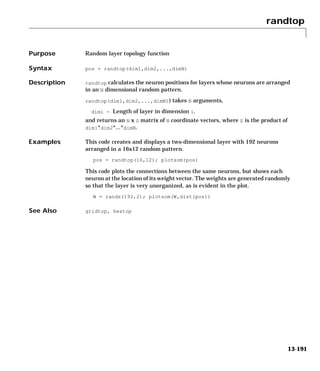
![satlin
Purpose Saturating linear transfer function
satlin
Syntax A = satlin(N)
info = satlin(code)
Description satlin is a transfer function. Transfer functions calculate a layer's output from
its net input.
satlin(N) takes one input,
N - S x Q matrix of net input (column) vectors,
and returns values of N truncated into the interval [-1, 1].
satlin(code) returns useful information for each code string:
'deriv' - Name of derivative function.
'name' - Full name.
'output' - Output range.
'active' - Active input range.
Examples Here is the code to create a plot of the satlin transfer function.
n = -5:0.1:5;
a = satlin(n);
plot(n,a)
Network Use To change a network so that a layer uses satlin, set
net.layers{i}.transferFcn to 'satlin'.
Call sim to simulate the network with satlin. See newhop for simulation
examples.
Algorithm satlin(n) = 0, if n <= 0; n, if 0 <= n <= 1; 1, if 1 <= n.
See Also sim, poslin, satlins, purelin
13-192](https://image.slidesharecdn.com/nnet-090922002848-phpapp01/85/Neural-Network-Toolbox-MATLAB-594-320.jpg)
![satlins
Purpose Symmetric saturating linear transfer function
satlins
Syntax A = satlins(N)
info = satlins(code)
Description satlins is a transfer function. Transfer functions calculate a layer's output
from its net input.
satlins(N) takes one input,
N - S x Q matrix of net input (column) vectors.
and returns values of N truncated into the interval [-1, 1].
satlins(code) returns useful information for each code string:
'deriv' - Name of derivative function.
'name' - Full name.
'output' - Output range.
'active' - Active input range.
Examples Here is the code to create a plot of the satlins transfer function.
n = -5:0.1:5;
a = satlins(n);
plot(n,a)
Network Use You can create a standard network that uses satlins by calling newhop.
To change a network so that a layer uses satlins, set
net.layers{i}.transferFcn to 'satlins'.
In either case, call sim to simulate the network with satlins. See newhop for
simulation examples.
Algorithm satlins(n) = -1, if n <= -1; n, if -1 <= n <= 1; 1, if 1 <= n.
See Also sim, satlin, poslin, purelin
13-193](https://image.slidesharecdn.com/nnet-090922002848-phpapp01/85/Neural-Network-Toolbox-MATLAB-595-320.jpg)
![seq2con
Purpose Converts sequential vectors to concurrent vectors
seq2con
Syntax b = seq2con(s)
Description The neural network toolbox represents batches of vectors with a matrix, and
sequences of vectors with multiple columns of a cell array.
seq2con and con2seq allow concurrent vectors to be converted to sequential
vectors, and back again.
seq2con(S) takes one input,
S - N x TS cell array of matrices with M columns.
and returns,
B - N x 1 cell array of matrices with M*TS columns.
Examples Here three sequential values are converted to concurrent values.
p1 = {1 4 2}
p2 = seq2con(p1)
Here two sequences of vectors over three time steps are converted to concurrent
vectors.
p1 = {[1; 1] [5; 4] [1; 2]; [3; 9] [4; 1] [9; 8]}
p2 = seq2con(p1)
See Also con2seq, concur
13-194](https://image.slidesharecdn.com/nnet-090922002848-phpapp01/85/Neural-Network-Toolbox-MATLAB-596-320.jpg)
![sim
Purpose Simulate a neural network
sim
Syntax [Y,Pf,Af] = sim(net,P,Pi,Ai)
[Y,Pf,Af] = sim(net,{Q TS},Pi,Ai)
[Y,Pf,Af] = sim(net,Q,Pi,Ai)
To Get Help Type help network/sim
Description sim simulates neural networks.
[Y,Pf,Af] = sim(net,P,Pi,Ai) takes,
net - Network.
P - Network inputs.
Pi - Initial input delay conditions, default = zeros.
Ai - Initial layer delay conditions, default = zeros.
and returns,
Y - Network outputs.
Pf - Final input delay conditions.
Af - Final layer delay conditions.
Note that arguments Pi, Ai, Pf, and Af are optional and need only be used for
networks that have input or layer delays.
sim's signal arguments can have two formats: cell array or matrix.
The cell array format is easiest to describe. It is most convenient for networks
with multiple inputs and outputs, and allows sequences of inputs to be
presented:
P - Ni x TS cell array, each element P{i,ts} is an Ri x Q matrix.
Pi - Ni x ID cell array, each element Pi{i,k} is an Ri x Q matrix.
Ai - Nl x LD cell array, each element Ai{i,k} is an Si x Q matrix.
Y - NO x TS cell array, each element Y{i,ts} is a Ui x Q matrix.
Pf - Ni x ID cell array, each element Pf{i,k} is an Ri x Q matrix.
Af - Nl x LD cell array, each element Af{i,k} is an Si x Q matrix.
13-195](https://image.slidesharecdn.com/nnet-090922002848-phpapp01/85/Neural-Network-Toolbox-MATLAB-597-320.jpg)
![sim
[Y,Pf,Af] = sim(net,{Q TS},Pi,Ai) is used for networks which do not have
an input, such as Hopfield networks, when cell array notation is used.
[Y,Pf,Af] = sim(net,Q,Pi,Ai) is used for networks which do not have an
input, such as Hopfield networks, when matrix notation is used.
Examples Here newp is used to create a perceptron layer with a 2-element input (with
ranges of [0 1]), and a single neuron.
net = newp([0 1;0 1],1);
Here the perceptron is simulated for an individual vector, a batch of 3 vectors,
and a sequence of 3 vectors.
p1 = [.2; .9]; a1 = sim(net,p1)
p2 = [.2 .5 .1; .9 .3 .7]; a2 = sim(net,p2)
p3 = {[.2; .9] [.5; .3] [.1; .7]}; a3 = sim(net,p3)
Here newlind is used to create a linear layer with a 3-element input, 2 neurons.
net = newlin([0 2;0 2;0 2],2,[0 1]);
Here the linear layer is simulated with a sequence of 2 input vectors using the
default initial input delay conditions (all zeros).
p1 = {[2; 0.5; 1] [1; 1.2; 0.1]};
[y1,pf] = sim(net,p1)
Here the layer is simulated for 3 more vectors using the previous final input
delay conditions as the new initial delay conditions.
p2 = {[0.5; 0.6; 1.8] [1.3; 1.6; 1.1] [0.2; 0.1; 0]};
[y2,pf] = sim(net,p2,pf)
Here newelm is used to create an Elman network with a 1-element input, and
a layer 1 with 3 tansig neurons followed by a layer 2 with 2 purelin neurons.
Because it is an Elman network it has a tap delay line with a delay of 1 going
from layer 1 to layer 1.
net = newelm([0 1],[3 2],{'tansig','purelin'});
13-197](https://image.slidesharecdn.com/nnet-090922002848-phpapp01/85/Neural-Network-Toolbox-MATLAB-599-320.jpg)
![sim
Here the Elman network is simulated for a sequence of 3 values using default
initial delay conditions.
p1 = {0.2 0.7 0.1};
[y1,pf,af] = sim(net,p1)
Here the network is simulated for 4 more values, using the previous final delay
conditions as the new initial delay conditions.
p2 = {0.1 0.9 0.8 0.4};
[y2,pf,af] = sim(net,p2,pf,af)
Algorithm sim uses these properties to simulate a network net.
net.numInputs, net.numLayers
net.outputConnect, net.biasConnect
net.inputConnect, net.layerConnect
These properties determine the network's weight and bias values, and the
number of delays associated with each weight:
net.inputWeights{i,j}.value
net.layerWeights{i,j}.value
net.layers{i}.value
net.inputWeights{i,j}.delays
net.layerWeights{i,j}.delays
These function properties indicate how sim applies weight and bias values to
inputs to get each layer's output:
net.inputWeights{i,j}.weightFcn
net.layerWeights{i,j}.weightFcn
net.layers{i}.netInputFcn
net.layers{i}.transferFcn
See Chapter 2 for more information on network simulation.
See Also init, adapt, train
13-198](https://image.slidesharecdn.com/nnet-090922002848-phpapp01/85/Neural-Network-Toolbox-MATLAB-600-320.jpg)
![softmax
Purpose Soft max transfer function
softmax
Syntax A = softmax(N)
info = softmax(code)
Description softmax is a transfer function. Transfer functions calculate a layer's output
from its net input.
softmax(N) takes one input argument,
N - S x Q matrix of net input (column) vectors.
and returns output vectors with elements between 0 and 1, but with their size
relations intact.
softmax('code') returns information about this function.
These codes are defined:
'deriv' - Name of derivative function.
'name' - Full name.
'output' - Output range.
'active' - Active input range.
compet does not have a derivative function.
Examples Here we define a net input vector N, calculate the output, and plot both with
bar graphs.
n = [0; 1; -0.5; 0.5];
a = softmax(n);
subplot(2,1,1), bar(n), ylabel('n')
subplot(2,1,2), bar(a), ylabel('a')
Network Use To change a network so that a layer uses softmax, set
net.layers{i,j}.transferFcn to 'softmax'.
Call sim to simulate the network with softmax. See newc or newpnn for
simulation examples.
See Also sim, compet
13-199](https://image.slidesharecdn.com/nnet-090922002848-phpapp01/85/Neural-Network-Toolbox-MATLAB-601-320.jpg)
![srchbac
Purpose One-dimensional minimization using backtracking
srchbac
Syntax [a,gX,perf,retcode,delta,tol] =
srchbac(net,X,Pd,Tl,Ai,Q,TS,dX,gX,perf,dperf,delta,tol,ch_perf)
Description srchbac is a linear search routine. It searches in a given direction to locate the
minimum of the performance function in that direction. It uses a technique
called backtracking.
srchbac(net,X,Pd,Tl,Ai,Q,TS,dX,gX,perf,dperf,delta,TOL,ch_perf)
takes these inputs,
net - Neural network.
X - Vector containing current values of weights and biases.
Pd - Delayed input vectors.
Tl - Layer target vectors.
Ai - Initial input delay conditions.
Q - Batch size.
TS - Time steps.
dX - Search direction vector.
gX - Gradient vector.
perf - Performance value at current X.
dperf - Slope of performance value at current X in direction of dX.
delta - Initial step size.
tol - Tolerance on search.
ch_perf - Change in performance on previous step.
and returns,
A - Step size which minimizes performance.
gX - Gradient at new minimum point.
perf - Performance value at new minimum point.
retcode - Return code which has three elements. The first two elements
correspond to the number of function evaluations in the two stages of the
search. The third element is a return code. These will have different
13-200](https://image.slidesharecdn.com/nnet-090922002848-phpapp01/85/Neural-Network-Toolbox-MATLAB-602-320.jpg)

![srchbac
Examples Here is a problem consisting of inputs P and targets T that we would like to
solve with a network.
P = [0 1 2 3 4 5];
T = [0 0 0 1 1 1];
Here a two-layer feed-forward network is created. The network's input ranges
from [0 to 10]. The first layer has two tansig neurons, and the second layer
has one logsig neuron. The traincgf network training function and the
srchbac search function are to be used.
Create and Test a Network
net = newff([0 5],[2 1],{'tansig','logsig'},'traincgf');
a = sim(net,p)
Train and Retest the Network
net.trainParam.searchFcn = 'srchbac';
net.trainParam.epochs = 50;
net.trainParam.show = 10;
net.trainParam.goal = 0.1;
net = train(net,p,t);
a = sim(net,p)
Network Use You can create a standard network that uses srchbac with newff, newcf, or
newelm.
To prepare a custom network to be trained with traincgf, using the line
search function srchbac:
1 Set net.trainFcn to 'traincgf'. This will set net.trainParam to traincgf's
default parameters.
2 Set net.trainParam.searchFcn to 'srchbac'.
The srchbac function can be used with any of the following training functions:
traincgf, traincgb, traincgp, trainbfg, trainoss.
13-202](https://image.slidesharecdn.com/nnet-090922002848-phpapp01/85/Neural-Network-Toolbox-MATLAB-604-320.jpg)
![srchbre
Purpose One-dimensional interval location using Brent's method
srchbre
Syntax [a,gX,perf,retcode,delta,tol] =
srchbre(net,X,Pd,Tl,Ai,Q,TS,dX,gX,perf,dperf,delta,tol,ch_perf)
Description srchbre is a linear search routine. It searches in a given direction to locate the
minimum of the performance function in that direction. It uses a technique
called Brent’s technique.
srchbre(net,X,Pd,Tl,Ai,Q,TS,dX,gX,perf,dperf,delta,tol,ch_perf)
takes these inputs,
net - Neural network.
X - Vector containing current values of weights and biases.
Pd - Delayed input vectors.
Tl - Layer target vectors.
Ai - Initial input delay conditions.
Q - Batch size.
TS - Time steps.
dX - Search direction vector.
gX - Gradient vector.
perf - Performance value at current X.
dperf - Slope of performance value at current X in direction of dX.
delta - Initial step size.
tol - Tolerance on search.
ch_perf - Change in performance on previous step.
and returns,
A - Step size which minimizes performance.
gX - Gradient at new minimum point.
perf - Performance value at new minimum point.
retcode - Return code, which has three elements. The first two elements
correspond to the number of function evaluations in the two stages of the
search. The third element is a return code. These will have different
13-204](https://image.slidesharecdn.com/nnet-090922002848-phpapp01/85/Neural-Network-Toolbox-MATLAB-606-320.jpg)
![srchbre
meanings for different search algorithms. Some may not be used in this
function.
0 - normal; 1 - minimum step taken;
2 - maximum step taken; 3 - beta condition not met.
delta - New initial step size. Based on the current step size.
tol - New tolerance on search.
Parameters used for the brent algorithm are:
alpha - Scale factor which determines sufficient reduction in perf.
beta - Scale factor which determines sufficiently large step size.
bmax - Largest step size.
scale_tol - Parameter which relates the tolerance tol to the initial step
size delta. Usually set to 20.
The defaults for these parameters are set in the training function which calls
it. See traincgf, traincgb, traincgp, trainbfg, trainoss.
Dimensions for these variables are:
Pd - No x Ni x TS cell array, each element P{i,j,ts} is a Dij x Q matrix.
Tl - Nl x TS cell array, each element P{i,ts} is an Vi x Q matrix.
Ai - Nl x LD cell array, each element Ai{i,k} is an Si x Q matrix.
where
Ni = net.numInputs
Nl = net.numLayers
LD = net.numLayerDelays
Ri = net.inputs{i}.size
Si = net.layers{i}.size
Vi = net.targets{i}.size
Dij = Ri * length(net.inputWeights{i,j}.delays)
Examples Here is a problem consisting of inputs P and targets T that we would like to
solve with a network.
P = [0 1 2 3 4 5];
T = [0 0 0 1 1 1];
13-205](https://image.slidesharecdn.com/nnet-090922002848-phpapp01/85/Neural-Network-Toolbox-MATLAB-607-320.jpg)
![srchbre
Here a two-layer feed-forward network is created. The network's input ranges
from [0 to 10]. The first layer has two tansig neurons, and the second layer
has one logsig neuron. The traincgf network training function and the
srchbac search function are to be used.
Create and Test a Network
net = newff([0 5],[2 1],{'tansig','logsig'},'traincgf');
a = sim(net,p)
Train and Retest the Network
net.trainParam.searchFcn = 'srchbre';
net.trainParam.epochs = 50;
net.trainParam.show = 10;
net.trainParam.goal = 0.1;
net = train(net,p,t);
a = sim(net,p)
Network Use You can create a standard network that uses srchbre with newff, newcf, or
newelm.
To prepare a custom network to be trained with traincgf, using the line
search function srchbre:
1 Set net.trainFcn to 'traincgf'. This will set net.trainParam to traincgf's
default parameters.
2 Set net.trainParam.searchFcn to 'srchbre'.
The srchbre function can be used with any of the following training functions:
traincgf, traincgb, traincgp, trainbfg, trainoss.
Algorithm srchbre brackets the minimum of the performance function in the search
direction dX, using Brent's algorithm described on page 46 of Scales
(Introduction to Non-Linear Estimation 1985). It is a hybrid algorithm based
on the golden section search and the quadratic approximation.
See Also srchbac, srchcha, srchgol, srchhyb
References Scales, L. E., Introduction to Non-Linear Optimization, New York:
Springer-Verlag, 1985.
13-206](https://image.slidesharecdn.com/nnet-090922002848-phpapp01/85/Neural-Network-Toolbox-MATLAB-608-320.jpg)
![srchcha
Purpose One-dimensional minimization using the method of Charalambous
srchcha
Syntax [a,gX,perf,retcode,delta,tol] =
srchcha(net,X,Pd,Tl,Ai,Q,TS,dX,gX,perf,dperf,delta,tol,ch_perf)
Description srchcha is a linear search routine. It searches in a given direction to locate the
minimum of the performance function in that direction. It uses a technique
based on the method of Charalambous.
srchcha(net,X,Pd,Tl,Ai,Q,TS,dX,gX,perf,dperf,delta,tol,ch_perf)
takes these inputs,
net - Neural network.
X - Vector containing current values of weights and biases.
Pd - Delayed input vectors.
Tl - Layer target vectors.
Ai - Initial input delay conditions.
Q - Batch size.
TS - Time steps.
dX - Search direction vector.
gX - Gradient vector.
perf - Performance value at current X.
dperf - Slope of performance value at current X in direction of dX.
delta - Initial step size.
tol - Tolerance on search.
ch_perf - Change in performance on previous step.
and returns,
A - Step size which minimizes performance.
gX - Gradient at new minimum point.
perf - Performance value at new minimum point.
retcode - Return code, which has three elements. The first two elements
correspond to the number of function evaluations in the two stages of the
search. The third element is a return code. These will have different
13-207](https://image.slidesharecdn.com/nnet-090922002848-phpapp01/85/Neural-Network-Toolbox-MATLAB-609-320.jpg)
![srchcha
meanings for different search algorithms. Some may not be used in this
function.
0 - normal; 1 - minimum step taken;
2 - maximum step taken; 3 - beta condition not met.
delta - New initial step size. Based on the current step size.
TOL - New tolerance on search.
Parameters used for the Charalambous algorithm are:
alpha - Scale factor which determines sufficient reduction in perf.
beta - Scale factor which determines sufficiently large step size.
gama - Parameter to avoid small reductions in performance. Usually set to 0.1.
scale_tol - Parameter which relates the tolerance tol to the initial step
size delta. Usually set to 20.
The defaults for these parameters are set in the training function which calls
it. See traincgf, traincgb, traincgp, trainbfg, trainoss.
Dimensions for these variables are:
Pd - No x Ni x TS cell array, each element P{i,j,ts} is a Dij x Q matrix.
Tl - Nl x TS cell array, each element P{i,ts} is an Vi x Q matrix.
Ai - Nl x LD cell array, each element Ai{i,k} is an Si x Q matrix.
where
Ni = net.numInputs
Nl = net.numLayers
LD = net.numLayerDelays
Ri = net.inputs{i}.size
Si = net.layers{i}.size
Vi = net.targets{i}.size
Dij = Ri * length(net.inputWeights{i,j}.delays)
Examples Here is a problem consisting of inputs P and targets T that we would like to
solve with a network.
P = [0 1 2 3 4 5];
T = [0 0 0 1 1 1];
13-208](https://image.slidesharecdn.com/nnet-090922002848-phpapp01/85/Neural-Network-Toolbox-MATLAB-610-320.jpg)
![srchcha
Here a two-layer feed-forward network is created. The network's input ranges
from [0 to 10]. The first layer has two tansig neurons, and the second layer
has one logsig neuron. The traincgf network training function and the
srchcha search function are to be used.
Create and Test a Network
net = newff([0 5],[2 1],{'tansig','logsig'},'traincgf');
a = sim(net,p)
Train and Retest the Network
net.trainParam.searchFcn = 'srchcha';
net.trainParam.epochs = 50;
net.trainParam.show = 10;
net.trainParam.goal = 0.1;
net = train(net,p,t);
a = sim(net,p)
Network Use You can create a standard network that uses srchcha with newff, newcf, or
newelm.
To prepare a custom network to be trained with traincgf, using the line search
function srchcha:
1 Set net.trainFcn to 'traincgf'. This will set net.trainParam to traincgf's
default parameters.
2 Set net.trainParam.searchFcn to 'srchcha'.
The srchcha function can be used with any of the following training functions:
traincgf, traincgb, traincgp, trainbfg, trainoss.
Algorithm srchcha locates the minimum of the performance function in the search
direction dX, using an algorithm based on the method described in
Charalambous (IEEE Proc. vol. 139, no. 3, June 1992).
See Also srchbac, srchbre, srchgol, srchhyb
References Charalambous, C.,“Conjugate gradient algorithm for efficient training of
artificial neural networks,” IEEE Proceedings, vol. 139, no. 3, pp. 301–310,
1992.
13-209](https://image.slidesharecdn.com/nnet-090922002848-phpapp01/85/Neural-Network-Toolbox-MATLAB-611-320.jpg)
![srchgol
Purpose One-dimensional minimization using golden section search
srchgol
Syntax [a,gX,perf,retcode,delta,tol] =
srchgol(net,X,Pd,Tl,Ai,Q,TS,dX,gX,perf,dperf,delta,tol,ch_perf)
Description srchgol is a linear search routine. It searches in a given direction to locate the
minimum of the performance function in that direction. It uses a technique
called the golden section search.
srchgol(net,X,Pd,Tl,Ai,Q,TS,dX,gX,perf,dperf,delta,tol,ch_perf)
takes these inputs,
net - Neural network.
X - Vector containing current values of weights and biases.
Pd - Delayed input vectors.
Tl - Layer target vectors.
Ai - Initial input delay conditions.
Q - Batch size.
TS - Time steps.
dX - Search direction vector.
gX - Gradient vector.
perf - Performance value at current X.
dperf - Slope of performance value at current X in direction of dX.
delta - Initial step size.
tol - Tolerance on search.
ch_perf - Change in performance on previous step.
and returns,
A - Step size which minimizes performance.
gX - Gradient at new minimum point.
perf - Performance value at new minimum point.
retcode - Return code, which has three elements. The first two elements
correspond to the number of function evaluations in the two stages of the
search. The third element is a return code. These will have different
13-210](https://image.slidesharecdn.com/nnet-090922002848-phpapp01/85/Neural-Network-Toolbox-MATLAB-612-320.jpg)
![srchgol
meanings for different search algorithms. Some may not be used in this
function.
0 - normal; 1 - minimum step taken;
2 - maximum step taken; 3 - beta condition not met.
delta - New initial step size. Based on the current step size.
tol - New tolerance on search.
Parameters used for the golden section algorithm are:
alpha - Scale factor which determines sufficient reduction in perf.
bmax - Largest step size.
scale_tol - Parameter which relates the tolerance tol to the initial step
size delta. Usually set to 20.
The defaults for these parameters are set in the training function which calls
it. See traincgf, traincgb, traincgp, trainbfg, trainoss.
Dimensions for these variables are:
Pd - No x Ni x TS cell array, each element P{i,j,ts} is a Dij x Q matrix.
Tl - Nl x TS cell array, each element P{i,ts} is an Vi x Q matrix.
Ai - Nl x LD cell array, each element Ai{i,k} is an Si x Q matrix.
where
Ni = net.numInputs
Nl = net.numLayers
LD = net.numLayerDelays
Ri = net.inputs{i}.size
Si = net.layers{i}.size
Vi = net.targets{i}.size
Dij = Ri * length(net.inputWeights{i,j}.delays)
Examples Here is a problem consisting of inputs P and targets T that we would like to
solve with a network.
P = [0 1 2 3 4 5];
T = [0 0 0 1 1 1];
13-211](https://image.slidesharecdn.com/nnet-090922002848-phpapp01/85/Neural-Network-Toolbox-MATLAB-613-320.jpg)
![srchgol
Here a two-layer feed-forward network is created. The network's input ranges
from [0 to 10]. The first layer has two tansig neurons, and the second layer
has one logsig neuron. The traincgf network training function and the
srchgol search function are to be used.
Create and Test a Network
net = newff([0 5],[2 1],{'tansig','logsig'},'traincgf');
a = sim(net,p)
Train and Retest the Network
net.trainParam.searchFcn = 'srchgol';
net.trainParam.epochs = 50;
net.trainParam.show = 10;
net.trainParam.goal = 0.1;
net = train(net,p,t);
a = sim(net,p)
Network Use You can create a standard network that uses srchgol with newff, newcf, or
newelm.
To prepare a custom network to be trained with traincgf, using the line search
function srchgol:
1 Set net.trainFcn to 'traincgf'. This will set net.trainParam to traincgf's
default parameters.
2 Set net.trainParam.searchFcn to 'srchgol'.
The srchgol function can be used with any of the following training functions:
traincgf, traincgb, traincgp, trainbfg, trainoss.
Algorithm srchgol locates the minimum of the performance function in the search
direction dX, using the golden section search. It is based on the algorithm as
described on page 33 of Scales (Introduction to Non-Linear Estimation 1985).
See Also srchbac, srchbre, srchcha, srchhyb
References Scales, L. E.,Introduction to Non-Linear Optimization, New York:
Springer-Verlag, 1985.
13-212](https://image.slidesharecdn.com/nnet-090922002848-phpapp01/85/Neural-Network-Toolbox-MATLAB-614-320.jpg)
![srchhyb
Purpose One-dimensional minimization using a hybrid bisection-cubic search
srchhyb
Syntax [a,gX,perf,retcode,delta,tol] =
srchhyb(net,X,P,T,Q,TS,dX,gX,perf,dperf,delta,tol,ch_perf)
Description srchhyb is a linear search routine. It searches in a given direction to locate the
minimum of the performance function in that direction. It uses a technique
that is a combination of a bisection and a cubic interpolation.
srchhyb(net,X,Pd,Tl,Ai,Q,TS,dX,gX,perf,dperf,delta,tol,ch_perf)
takes these inputs,
net - Neural network.
X - Vector containing current values of weights and biases.
Pd - Delayed input vectors.
Tl - Layer target vectors.
Ai - Initial input delay conditions.
Q - Batch size.
TS - Time steps.
dX - Search direction vector.
gX - Gradient vector.
perf - Performance value at current X.
dperf - Slope of performance value at current X in direction of dX.
delta - Initial step size.
tol - Tolerance on search.
ch_perf - Change in performance on previous step.
and returns,
A - Step size which minimizes performance.
gX - Gradient at new minimum point.
perf - Performance value at new minimum point.
retcode - Return code, which has three elements. The first two elements
correspond to the number of function evaluations in the two stages of the
search. The third element is a return code. These will have different
13-213](https://image.slidesharecdn.com/nnet-090922002848-phpapp01/85/Neural-Network-Toolbox-MATLAB-615-320.jpg)
![srchhyb
meanings for different search algorithms. Some may not be used in this
function.
0 - normal; 1 - minimum step taken;
2 - maximum step taken; 3 - beta condition not met.
delta - New initial step size. Based on the current step size.
tol - New tolerance on search.
Parameters used for the hybrid bisection-cubic algorithm are:
alpha - Scale factor which determines sufficient reduction in perf.
beta - Scale factor which determines sufficiently large step size.
bmax - Largest step size.
scale_tol - Parameter which relates the tolerance tol to the initial step
size delta. Usually set to 20.
The defaults for these parameters are set in the training function which calls
it. See traincgf, traincgb, traincgp, trainbfg, trainoss.
Dimensions for these variables are:
Pd - No x Ni x TS cell array, each element P{i,j,ts} is a Dij x Q matrix.
Tl - Nl x TS cell array, each element P{i,ts} is an Vi x Q matrix.
Ai - Nl x LD cell array, each element Ai{i,k} is an Si x Q matrix.
where
Ni = net.numInputs
Nl = net.numLayers
LD = net.numLayerDelays
Ri = net.inputs{i}.size
Si = net.layers{i}.size
Vi = net.targets{i}.size
Dij = Ri * length(net.inputWeights{i,j}.delays)
Examples Here is a problem consisting of inputs P and targets T that we would like to
solve with a network.
P = [0 1 2 3 4 5];
T = [0 0 0 1 1 1];
13-214](https://image.slidesharecdn.com/nnet-090922002848-phpapp01/85/Neural-Network-Toolbox-MATLAB-616-320.jpg)
![srchhyb
Here a two-layer feed-forward network is created. The network's input ranges
from [0 to 10]. The first layer has two tansig neurons, and the second layer
has one logsig neuron. The traincgf network training function and the
srchhyb search function are to be used.
Create and Test a Network
net = newff([0 5],[2 1],{'tansig','logsig'},'traincgf');
a = sim(net,p)
Train and Retest the Network
net.trainParam.searchFcn = 'srchhyb';
net.trainParam.epochs = 50;
net.trainParam.show = 10;
net.trainParam.goal = 0.1;
net = train(net,p,t);
a = sim(net,p)
Network Use You can create a standard network that uses srchhyb with newff, newcf, or
newelm.
To prepare a custom network to be trained with traincgf, using the line search
function srchhyb:
1 Set net.trainFcn to 'traincgf'. This will set net.trainParam to traincgf's
default parameters.
2 Set net.trainParam.searchFcn to 'srchhyb'.
The srchhyb function can be used with any of the following training functions:
traincgf, traincgb, traincgp, trainbfg, trainoss.
Algorithm srchhyb locates the minimum of the performance function in the search
direction dX, using the hybrid bisection-cubic interpolation algorithm described
on page 50 of Scales (Introduction to Non-Linear Estimation 1985).
See Also srchbac, srchbre, srchcha, srchgol
References Scales, L. E., Introduction to Non-Linear Optimization, New York:
Springer-Verlag, 1985.
13-215](https://image.slidesharecdn.com/nnet-090922002848-phpapp01/85/Neural-Network-Toolbox-MATLAB-617-320.jpg)
![sse
Purpose Sum squared error performance function
sse
Syntax perf = sse(e,x,pp)
perf = sse(e,net,pp)
info = sse(code)
Description sse is a network performance function. It measures performance according to
the sum of squared errors.
sse(E,X,PP) takes from one to three arguments,
E - Matrix or cell array of error vector(s).
X - Vector of all weight and bias values (ignored).
PP - Performance parameters (ignored).
and returns the sum squared error.
sse(E,net,PP) can take an alternate argument to X,
net - Neural network from which X can be obtained (ignored).
sse(code) returns useful information for each code string:
'deriv' - Name of derivative function.
'name' - Full name.
'pnames' - Names of training parameters.
'pdefaults' - Default training parameters.
Examples Here a two layer feed-forward is created with a 1-element input ranging from
-10 to 10, four hidden tansig neurons, and one purelin output neuron.
net = newff([-10 10],[4 1],{'tansig','purelin'});
Here the network is given a batch of inputs P. The error is calculated by
subtracting the output A from target T. Then the sum squared error is
calculated.
13-216](https://image.slidesharecdn.com/nnet-090922002848-phpapp01/85/Neural-Network-Toolbox-MATLAB-618-320.jpg)
![sse
p = [-10 -5 0 5 10];
t = [0 0 1 1 1];
y = sim(net,p)
e = t-y
perf = sse(e)
Note that sse can be called with only one argument because the other
arguments are ignored. sse supports those arguments to conform to the
standard performance function argument list.
Network Use To prepare a custom network to be trained with sse set net.performFcn to
'sse'. This will automatically set net.performParam to the empty matrix [], as
sse has no performance parameters.
Calling train or adapt will result in sse being used to calculate performance.
See Also dsse
13-217](https://image.slidesharecdn.com/nnet-090922002848-phpapp01/85/Neural-Network-Toolbox-MATLAB-619-320.jpg)
![sumsqr
Purpose Sum squared elements of a matrix
sumsqr
Syntax sumsqr(m)
Description sumsqr(M) returns the sum of the squared elements in M.
Examples s = sumsqr([1 2;3 4])
13-218](https://image.slidesharecdn.com/nnet-090922002848-phpapp01/85/Neural-Network-Toolbox-MATLAB-620-320.jpg)
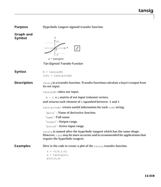
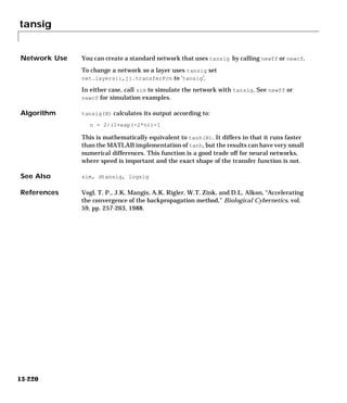
![train
Purpose Train a neural network
train
Syntax [net,tr] = train(NET,P,T,Pi,Ai)
[net,tr] = train(NET,P,T,Pi,Ai,VV,TV)
To Get Help Type help network/train
Description train trains a network net according to net.trainFcn and net.trainParam.
train(net,P,T,Pi,Ai) takes,
net - Network.
P - Network inputs.
T - Network targets, default = zeros.
Pi - Initial input delay conditions, default = zeros.
Ai - Initial layer delay conditions, default = zeros.
and returns,
net - New network.
TR - Training record (epoch and perf).
Note that T is optional and need only be used for networks that require targets.
Pi and Pf are also optional and need only be used for networks that have input
or layer delays.
train's signal arguments can have two formats: cell array or matrix.
The cell array format is easiest to describe. It is most convenient for networks
with multiple inputs and outputs, and allows sequences of inputs to be
presented:
P - Ni x TS cell array, each element P{i,ts} is an Ri x Q matrix.
T - Nt x TS cell array, each element P{i,ts} is an Vi x Q matrix.
Pi - Ni x ID cell array, each element Pi{i,k} is an Ri x Q matrix.
Ai - Nl x LD cell array, each element Ai{i,k} is an S i x Q matrix.
13-221](https://image.slidesharecdn.com/nnet-090922002848-phpapp01/85/Neural-Network-Toolbox-MATLAB-623-320.jpg)
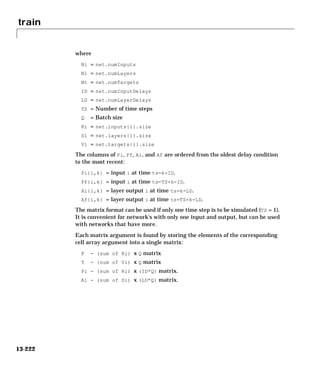
![train
train(net,P,T,Pi,Ai,VV,TV) takes optional structures of validation and test
vectors,
VV.P, TV.P - Validation/test inputs.
VV.T, VV.T - Validation/test targets, default = zeros.
VV.Pi, VV.Pi - Validation/test initial input delay conditions, default= zeros.
VV.Ai, VV.Ai - Validation/test layer delay conditions, default = zeros.
The validation vectors are used to stop training early if further training on the
primary vectors will hurt generalization to the validation vectors. Test vector
performance can be used to measure how well the network generalizes beyond
primary and validation vectors. If VV.T, VV.Pi, or VV.Ai are set to an empty
matrix or cell array, default values will be used. The same is true for VT.T,
VT.Pi, VT.Ai.
Examples Here input P and targets T define a simple function which we can plot:
p = [0 1 2 3 4 5 6 7 8];
t = [0 0.84 0.91 0.14 -0.77 -0.96 -0.28 0.66 0.99];
plot(p,t,'o')
Here newff is used to create a two layer feed forward network. The network
will have an input (ranging from 0 to 8), followed by a layer of 10 tansig
neurons, followed by a layer with 1 purelin neuron. trainlm backpropagation
is used. The network is also simulated.
net = newff([0 8],[10 1],{'tansig' 'purelin'},'trainlm');
y1 = sim(net,p)
plot(p,t,'o',p,y1,'x')
Here the network is trained for up to 50 epochs to a error goal of 0.01, and then
resimulated.
net.trainParam.epochs = 50;
net.trainParam.goal = 0.01;
net = train(net,p,t);
y2 = sim(net,p)
plot(p,t,'o',p,y1,'x',p,y2,'*')
Algorithm train calls the function indicated by net.trainFcn, using the adaption
parameter values indicated by net.trainParam.
13-223](https://image.slidesharecdn.com/nnet-090922002848-phpapp01/85/Neural-Network-Toolbox-MATLAB-625-320.jpg)
![trainbfg
Purpose BFGS quasi-Newton backpropagation
trainbfg
Syntax [net,tr] = trainbfg(net,Pd,Tl,Ai,Q,TS,VV)
info = trainbfg(code)
Description trainbfg is a network training function that updates weight and bias values
according to the BFGS quasi-Newton method.
trainbfg(net,Pd,Tl,Ai,Q,TS,VV,TV) takes these inputs,
net - Neural network.
Pd - Delayed input vectors.
Tl - Layer target vectors.
Ai - Initial input delay conditions.
Q - Batch size.
TS - Time steps.
VV - Either empty matrix [] or structure of validation vectors.
TV - Either empty matrix [] or structure of test vectors.
and returns,
net - Trained network.
TR - Training record of various values over each epoch:
TR.epoch - Epoch number.
TR.perf - Training performance.
TR.vperf - Validation performance.
TR.tperf - Test performance.
13-225](https://image.slidesharecdn.com/nnet-090922002848-phpapp01/85/Neural-Network-Toolbox-MATLAB-627-320.jpg)
![trainbfg
Dimensions for these variables are:
Pd - No x Ni x TS cell array, each element P{i,j,ts} is a Dij x Q matrix.
Tl - Nl x TS cell array, each element P{i,ts} is a Vi x Q matrix.
Ai - Nl x LD cell array, each element Ai{i,k} is an Si x Q matrix.
where
Ni = net.numInputs
Nl = net.numLayers
LD = net.numLayerDelays
Ri = net.inputs{i}.size
Si = net.layers{i}.size
Vi = net.targets{i}.size
Dij = Ri * length(net.inputWeights{i,j}.delays)
If VV is not [], it must be a structure of validation vectors,
VV.PD - Validation delayed inputs.
VV.Tl - Validation layer targets.
VV.Ai - Validation initial input conditions.
VV.Q - Validation batch size.
VV.TS - Validation time steps.
which is used to stop training early if the network performance on the
validation vectors fails to improve or remains the same for max_fail epochs in
a row.
If TV is not [], it must be a structure of validation vectors,
TV.PD - Validation delayed inputs.
TV.Tl - Validation layer targets.
TV.Ai - Validation initial input conditions.
TV.Q - Validation batch size.
TV.TS - Validation time steps.
which is used to test the generalization capability of the trained network.
13-227](https://image.slidesharecdn.com/nnet-090922002848-phpapp01/85/Neural-Network-Toolbox-MATLAB-629-320.jpg)
![trainbfg
trainbfg(code) returns useful information for each code string:
'pnames' - Names of training parameters.
'pdefaults' - Default training parameters.
Examples Here is a problem consisting of inputs P and targets T that we would like to
solve with a network.
P = [0 1 2 3 4 5];
T = [0 0 0 1 1 1];
Here a two-layer feed-forward network is created. The network's input ranges
from [0 to 10]. The first layer has two tansig neurons, and the second layer
has one logsig neuron. The trainbfg network training function is to be used.
Create and Test a Network
net = newff([0 5],[2 1],{'tansig','logsig'},'trainbfg');
a = sim(net,p)
Train and Retest the Network
net.trainParam.epochs = 50;
net.trainParam.show = 10;
net.trainParam.goal = 0.1;
net = train(net,p,t);
a = sim(net,p)
See newff, newcf, and newelm for other examples
Network Use You can create a standard network that uses trainbfg with newff, newcf, or
newelm.
To prepare a custom network to be trained with trainbfg:
1 Set net.trainFcn to 'trainbfg'. This will set net.trainParam to trainbfg's
default parameters.
2 Set net.trainParam properties to desired values.
In either case, calling train with the resulting network will train the network
with trainbfg.
13-228](https://image.slidesharecdn.com/nnet-090922002848-phpapp01/85/Neural-Network-Toolbox-MATLAB-630-320.jpg)
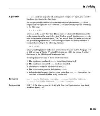
![trainbr
Purpose Bayesian Regulation backpropagation
trainbr
Syntax [net,tr] = trainbr(net,Pd,Tl,Ai,Q,TS,VV)
info = trainbr(code)
Description trainbr is a network training function that updates the weight and bias values
according to Levenberg-Marquardt optimization. It minimizes a combination of
squared errors and weights, and then determines the correct combination so as
to produce a network which generalizes well. The process is called Bayesian
regularization.
trainbr(net,Pd,Tl,Ai,Q,TS,VV,TV) takes these inputs,
net - Neural network.
Pd - Delayed input vectors.
Tl - Layer target vectors.
Ai - Initial input delay conditions.
Q - Batch size.
TS - Time steps.
VV - Either empty matrix [] or structure of validation vectors.
and returns,
net - Trained network.
TR - Training record of various values over each epoch:
TR.epoch - Epoch number.
TR.perf - Training performance.
TR.vperf - Validation performance.
TR.tperf - Test performance.
TR.mu - Adaptive mu value.
13-230](https://image.slidesharecdn.com/nnet-090922002848-phpapp01/85/Neural-Network-Toolbox-MATLAB-632-320.jpg)
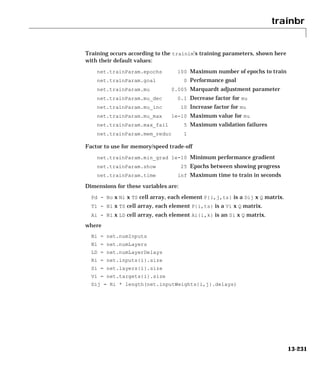
![trainbr
If VV is not [], it must be a structure of validation vectors,
VV.PD - Validation delayed inputs.
VV.Tl - Validation layer targets.
VV.Ai - Validation initial input conditions.
VV.Q - Validation batch size.
VV.TS - Validation time steps.
which is normally used to stop training early if the network performance on the
validation vectors fails to improve or remains the same for max_fail epochs in
a row. This early stopping is not used for trainbr, but the validation
performance is computed for analysis purposes if VV is not [].
trainbr(code) returns useful information for each code string:
'pnames' - Names of training parameters.
'pdefaults' - Default training parameters.
Examples Here is a problem consisting of inputs p and targets t that we would like to
solve with a network. It involves fitting a noisy sine wave.
p = [-1:.05:1];
t = sin(2*pi*p)+0.1*randn(size(p));
Here a two-layer feed-forward network is created. The network's input ranges
from [-1 to 1]. The first layer has 20 tansig neurons, the second layer has one
purelin neuron. The trainbr network training function is to be used. The plot
of the resulting network output should show a smooth response, without
overfitting.
Create a Network
net=newff([-1 1],[20,1],{'tansig','purelin'},'trainbr');
Train and Test the Network
net.trainParam.epochs = 50;
net.trainParam.show = 10;
net = train(net,p,t);
a = sim(net,p)
plot(p,a,p,t,'+')
13-232](https://image.slidesharecdn.com/nnet-090922002848-phpapp01/85/Neural-Network-Toolbox-MATLAB-634-320.jpg)
![traincgb
Purpose Conjugate gradient backpropagation with Powell-Beale restarts
traincgb
Syntax [net,tr] = traincgb(net,Pd,Tl,Ai,Q,TS,VV)
info = traincgb(code)
Description traincgb is a network training function that updates weight and bias values
according to the conjugate gradient backpropagation with Powell-Beale
restarts.
traincgb(net,Pd,Tl,Ai,Q,TS,VV,TV) takes these inputs,
net - Neural network.
Pd - Delayed input vectors.
Tl - Layer target vectors.
Ai - Initial input delay conditions.
Q - Batch size.
TS - Time steps.
VV - Either empty matrix [] or structure of validation vectors.
TV - Either empty matrix [] or structure of test vectors.
and returns,
net - Trained network.
TR - Training record of various values over each epoch:
TR.epoch - Epoch number.
TR.perf - Training performance.
TR.vperf - Validation performance.
TR.tperf - Test performance.
13-235](https://image.slidesharecdn.com/nnet-090922002848-phpapp01/85/Neural-Network-Toolbox-MATLAB-637-320.jpg)
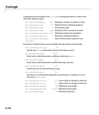
![traincgb
Dimensions for these variables are:
Pd - No x Ni x TS cell array, each element P{i,j,ts} is a Dij x Q matrix.
Tl - Nl x TS cell array, each element P{i,ts} is a Vi x Q matrix.
Ai - Nl x LD cell array, each element Ai{i,k} is an Si x Q matrix.
where
Ni = net.numInputs
Nl = net.numLayers
LD = net.numLayerDelays
Ri = net.inputs{i}.size
Si = net.layers{i}.size
Vi = net.targets{i}.size
Dij = Ri * length(net.inputWeights{i,j}.delays)
If VV is not [], it must be a structure of validation vectors,
VV.PD - Validation delayed inputs.
VV.Tl - Validation layer targets.
VV.Ai - Validation initial input conditions.
VV.Q - Validation batch size.
VV.TS - Validation time steps.
which is used to stop training early if the network performance on the
validation vectors fails to improve or remains the same for max_fail epochs in
a row.
If TV is not [], it must be a structure of validation vectors,
TV.PD - Validation delayed inputs.
TV.Tl - Validation layer targets.
TV.Ai - Validation initial input conditions.
TV.Q - Validation batch size.
TV.TS - Validation time steps.
which is used to test the generalization capability of the trained network.
13-237](https://image.slidesharecdn.com/nnet-090922002848-phpapp01/85/Neural-Network-Toolbox-MATLAB-639-320.jpg)
![traincgb
traincgb(code) returns useful information for each code string:
'pnames' - Names of training parameters.
'pdefaults' - Default training parameters.
Examples Here is a problem consisting of inputs P and targets T that we would like to
solve with a network.
P = [0 1 2 3 4 5];
T = [0 0 0 1 1 1];
Here a two-layer feed-forward network is created. The network's input ranges
from [0 to 10]. The first layer has two tansig neurons, and the second layer
has one logsig neuron. The traincgb network training function is to be used.
Create and Test a Network
net = newff([0 5],[2 1],{'tansig','logsig'},'traincgb');
a = sim(net,p)
Train and Retest the Network
net.trainParam.epochs = 50;
net.trainParam.show = 10;
net.trainParam.goal = 0.1;
net = train(net,p,t);
a = sim(net,p)
See newff, newcf, and newelm for other examples.
Network Use You can create a standard network that uses traincgb with newff, newcf, or
newelm.
To prepare a custom network to be trained with traincgb:
1 Set net.trainFcn to 'traincgb'. This will set net.trainParam to traincgb's
default parameters.
2 Set net.trainParam properties to desired values.
In either case, calling train with the resulting network will train the network
with traincgb.
13-238](https://image.slidesharecdn.com/nnet-090922002848-phpapp01/85/Neural-Network-Toolbox-MATLAB-640-320.jpg)
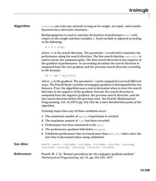
![traincgf
Purpose Conjugate gradient backpropagation with Fletcher-Reeves updates
traincgf
Syntax [net,tr] = traincgf(net,Pd,Tl,Ai,Q,TS,VV)
info = traincgf(code)
Description traincgf is a network training function that updates weight and bias values
according to the conjugate gradient backpropagation with Fletcher-Reeves
updates.
traincgf(net,Pd,Tl,Ai,Q,TS,VV,TV) takes these inputs,
net - Neural network.
Pd - Delayed input vectors.
Tl - Layer target vectors.
Ai - Initial input delay conditions.
Q - Batch size.
TS - Time steps.
VV - Either empty matrix [] or structure of validation vectors.
TV - Either empty matrix [] or structure of test vectors.
and returns,
net - Trained network.
TR - Training record of various values over each epoch:
TR.epoch - Epoch number.
TR.perf - Training performance.
TR.vperf - Validation performance.
TR.tperf - Test performance.
13-240](https://image.slidesharecdn.com/nnet-090922002848-phpapp01/85/Neural-Network-Toolbox-MATLAB-642-320.jpg)

![traincgf
Dimensions for these variables are:
Pd - No x Ni x TS cell array, each element P{i,j,ts} is a Dij x Q matrix.
Tl - Nl x TS cell array, each element P{i,ts} is a Vi x Q matrix.
Ai - Nl x LD cell array, each element Ai{i,k} is an Si x Q matrix.
where
Ni = net.numInputs
Nl = net.numLayers
LD = net.numLayerDelays
Ri = net.inputs{i}.size
Si = net.layers{i}.size
Vi = net.targets{i}.size
Dij = Ri * length(net.inputWeights{i,j}.delays)
If VV is not [], it must be a structure of validation vectors,
VV.PD - Validation delayed inputs.
VV.Tl - Validation layer targets.
VV.Ai - Validation initial input conditions.
VV.Q - Validation batch size.
VV.TS - Validation time steps.
which is used to stop training early if the network performance on the
validation vectors fails to improve or remains the same for max_fail epochs in
a row.
If TV is not [], it must be a structure of validation vectors,
TV.PD - Validation delayed inputs.
TV.Tl - Validation layer targets.
TV.Ai - Validation initial input conditions.
TV.Q - Validation batch size.
TV.TS - Validation time steps.
which is used to test the generalization capability of the trained network.
13-242](https://image.slidesharecdn.com/nnet-090922002848-phpapp01/85/Neural-Network-Toolbox-MATLAB-644-320.jpg)
![traincgf
traincgf(code) returns useful information for each code string:
'pnames' - Names of training parameters.
'pdefaults' - Default training parameters.
Examples Here is a problem consisting of inputs P and targets T that we would like to
solve with a network.
P = [0 1 2 3 4 5];
T = [0 0 0 1 1 1];
Here a two-layer feed-forward network is created. The network's input ranges
from [0 to 10]. The first layer has two tansig neurons, and the second layer
has one logsig neuron. The traincgf network training function is to be used.
Create and Test a Network
net = newff([0 5],[2 1],{'tansig','logsig'},'traincgf');
a = sim(net,p)
Train and Retest the Network
net.trainParam.epochs = 50;
net.trainParam.show = 10;
net.trainParam.goal = 0.1;
net = train(net,p,t);
a = sim(net,p)
See newff, newcf, and newelm for other examples.
Network Use You can create a standard network that uses traincgf with newff, newcf, or
newelm.
To prepare a custom network to be trained with traincgf:
1 Set net.trainFcn to 'traincgf'. This will set net.trainParam to traincgf's
default parameters.
2 Set net.trainParam properties to desired values.
In either case, calling train with the resulting network will train the network
with traincgf.
13-243](https://image.slidesharecdn.com/nnet-090922002848-phpapp01/85/Neural-Network-Toolbox-MATLAB-645-320.jpg)
![traincgp
Purpose Conjugate gradient backpropagation with Polak-Ribiere updates
traincgp
Syntax [net,tr] = traincgp(net,Pd,Tl,Ai,Q,TS,VV)
info = traincgp(code)
Description traincgp is a network training function that updates weight and bias values
according to the conjugate gradient backpropagation with Polak-Ribiere
updates.
traincgp(net,Pd,Tl,Ai,Q,TS,VV,TV) takes these inputs,
net - Neural network.
Pd - Delayed input vectors.
Tl - Layer target vectors.
Ai - Initial input delay conditions.
Q - Batch size.
TS - Time steps.
VV - Either empty matrix [] or structure of validation vectors.
TV - Either empty matrix [] or structure of test vectors.
and returns,
net - Trained network.
TR - Training record of various values over each epoch:
TR.epoch - Epoch number.
TR.perf - Training performance.
TR.vperf - Validation performance.
TR.tperf - Test performance.
13-246](https://image.slidesharecdn.com/nnet-090922002848-phpapp01/85/Neural-Network-Toolbox-MATLAB-648-320.jpg)

![traincgp
Dimensions for these variables are:
Pd - No x Ni x TS cell array, each element P{i,j,ts} is a Dij x Q matrix.
Tl - Nl x TS cell array, each element P{i,ts} is a Vi x Q matrix.
Ai - Nl x LD cell array, each element Ai{i,k} is an Si x Q matrix.
where
Ni = net.numInputs
Nl = net.numLayers
LD = net.numLayerDelays
Ri = net.inputs{i}.size
Si = net.layers{i}.size
Vi = net.targets{i}.size
Dij = Ri * length(net.inputWeights{i,j}.delays)
If VV is not [], it must be a structure of validation vectors,
VV.PD - Validation delayed inputs.
VV.Tl - Validation layer targets.
VV.Ai - Validation initial input conditions.
VV.Q - Validation batch size.
VV.TS - Validation time steps.
which is used to stop training early if the network performance on the
validation vectors fails to improve or remains the same for max_fail epochs in
a row.
If TV is not [], it must be a structure of validation vectors,
TV.PD - Validation delayed inputs.
TV.Tl - Validation layer targets.
TV.Ai - Validation initial input conditions.
TV.Q - Validation batch size.
TV.TS - Validation time steps.
which is used to test the generalization capability of the trained network.
13-248](https://image.slidesharecdn.com/nnet-090922002848-phpapp01/85/Neural-Network-Toolbox-MATLAB-650-320.jpg)
![traincgp
traincgp(code) returns useful information for each code string:
'pnames' - Names of training parameters.
'pdefaults' - Default training parameters.
Examples Here is a problem consisting of inputs P and targets T that we would like to
solve with a network.
P = [0 1 2 3 4 5];
T = [0 0 0 1 1 1];
Here a two-layer feed-forward network is created. The network's input ranges
from [0 to 10]. The first layer has two tansig neurons, and the second layer
has one logsig neuron. The traincgp network training function is to be used.
Create and Test a Network
net = newff([0 5],[2 1],{'tansig','logsig'},'traincgp');
a = sim(net,p)
Train and Retest the Network
net.trainParam.epochs = 50;
net.trainParam.show = 10;
net.trainParam.goal = 0.1;
net = train(net,p,t);
a = sim(net,p)
See newff, newcf, and newelm for other examples.
Network Use You can create a standard network that uses traincgp with newff, newcf, or
newelm.
To prepare a custom network to be trained with traincgp:
1 Set net.trainFcn to 'traincgp'. This will set net.trainParam to traincgp's
default parameters.
2 Set net.trainParam properties to desired values.
In either case, calling train with the resulting network will train the network
with traincgp.
13-249](https://image.slidesharecdn.com/nnet-090922002848-phpapp01/85/Neural-Network-Toolbox-MATLAB-651-320.jpg)

![traingd
Purpose Gradient descent backpropagation
traingd
Syntax [net,tr] = traingd(net,Pd,Tl,Ai,Q,TS,VV)
info = traingd(code)
Description traingd is a network training function that updates weight and bias values
according to gradient descent.
traingd(net,Pd,Tl,Ai,Q,TS,VV) takes these inputs,
net - Neural network.
Pd - Delayed input vectors.
Tl - Layer target vectors.
Ai - Initial input delay conditions.
Q - Batch size.
TS - Time steps.
VV - Either an empty matrix [] or a structure of validation vectors.
and returns,
net - Trained network.
TR - Training record of various values over each epoch:
TR.epoch - Epoch number.
TR.perf - Training performance.
TR.vperf - Validation performance.
TR.tperf - Test performance.
Training occurs according to the traingd's training parameters shown here
with their default values:
net.trainParam.epochs 10 Maximum number of epochs to train
net.trainParam.goal 0 Performance goal
net.trainParam.lr 0.01 Learning rate
net.trainParam.max_fail 5 Maximum validation failures
net.trainParam.min_grad 1e-10 Minimum performance gradient
net.trainParam.show 25 Epochs between showing progress
net.trainParam.time inf Maximum time to train in seconds
13-252](https://image.slidesharecdn.com/nnet-090922002848-phpapp01/85/Neural-Network-Toolbox-MATLAB-654-320.jpg)
![traingd
Dimensions for these variables are:
Pd - No x Ni x TS cell array, each element P{i,j,ts} is a Dij x Q matrix.
Tl - Nl x TS cell array, each element P{i,ts} is an Vi x Q matrix.
Ai - Nl x LD cell array, each element Ai{i,k} is an Si x Q matrix.
where
Ni = net.numInputs
Nl = net.numLayers
LD = net.numLayerDelays
Ri = net.inputs{i}.size
Si = net.layers{i}.size
Vi = net.targets{i}.size
Dij = Ri * length(net.inputWeights{i,j}.delays)
If VV is not [], it must be a structure of validation vectors,
VV.PD - Validation delayed inputs.
VV.Tl - Validation layer targets.
VV.Ai - Validation initial input conditions.
VV.Q - Validation batch size.
VV.TS - Validation time steps.
which are used to stop training early if the network performance on the
validation vectors fails to improve or remain the same for max_fail epochs in
a row.
traingd(code) returns useful information for each code string:
'pnames' - Names of training parameters.
'pdefaults' - Default training parameters.
Network Use You can create a standard network that uses traingd with newff, newcf, or
newelm.
13-253](https://image.slidesharecdn.com/nnet-090922002848-phpapp01/85/Neural-Network-Toolbox-MATLAB-655-320.jpg)
![traingda
Purpose Gradient descent with adaptive lr backpropagation
traingda
Syntax [net,tr] = traingda(net,Pd,Tl,Ai,Q,TS,VV)
info = traingda(code)
Description traingda is a network training function that updates weight and bias values
according to gradient descent with adaptive learning rate.
traingda(NET,Pd,Tl,Ai,Q,TS,VV) takes these inputs,
net - Neural network.
Pd - Delayed input vectors.
Tl - Layer target vectors.
Ai - Initial input delay conditions.
Q - Batch size.
TS - Time steps.
VV - Either empty matrix [] or structure of validation vectors.
and returns,
net - Trained network.
TR - Training record of various values over each epoch:
TR.epoch - Epoch number.
TR.perf - Training performance.
TR.vperf - Validation performance.
TR.tperf - Test performance.
TR.lr - Adaptive learning rate.
13-255](https://image.slidesharecdn.com/nnet-090922002848-phpapp01/85/Neural-Network-Toolbox-MATLAB-657-320.jpg)
![traingda
Training occurs according to the traingda's training parameters, shown here
with their default values:
net.trainParam.epochs 10 Maximum number of epochs to train
net.trainParam.goal 0 Performance goal
net.trainParam.lr 0.01 Learning rate
net.trainParam.lr_inc 1.05 Ratio to increase learning rate
net.trainParam.lr_dec 0.7 Ratio to decrease learning rate
net.trainParam.max_fail 5 Maximum validation failures
net.trainParam.max_perf_inc 1.04 Maximum performance increase
net.trainParam.min_grad 1e-10 Minimum performance gradient
net.trainParam.show 25 Epochs between showing progress
net.trainParam.time inf Maximum time to train in seconds
Dimensions for these variables are:
Pd - No x Ni x TS cell array, each element P{i,j,ts} is a Dij x Q matrix.
Tl - Nl x TS cell array, each element P{i,ts} is a Vi x Q matrix.
Ai - Nl x LD cell array, each element Ai{i,k} is an Si x Q matrix.
where
Ni = net.numInputs
Nl = net.numLayers
LD = net.numLayerDelays
Ri = net.inputs{i}.size
Si = net.layers{i}.size
Vi = net.targets{i}.size
Dij = Ri * length(net.inputWeights{i,j}.delays)
If VV is not [], it must be a structure of validation vectors,
VV.PD - Validation delayed inputs.
VV.Tl - Validation layer targets.
VV.Ai - Validation initial input conditions.
VV.Q - Validation batch size.
VV.TS - Validation time steps.
13-256](https://image.slidesharecdn.com/nnet-090922002848-phpapp01/85/Neural-Network-Toolbox-MATLAB-658-320.jpg)
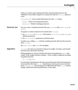
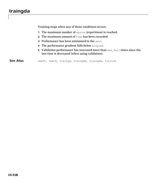
![traingdm
Purpose Gradient descent w/momentum backpropagation
traingdm
Syntax [net,tr] = traingdm(net,Pd,Tl,Ai,Q,TS,VV)
info = traingdm(code)
Description traingdm is a network training function that updates weight and bias values
according to gradient descent with adaptive learning rate.
traingdm(net,Pd,Tl,Ai,Q,TS,VV) takes these inputs,
net - Neural network.
Pd - Delayed input vectors.
Tl - Layer target vectors.
Ai - Initial input delay conditions.
Q - Batch size.
TS - Time steps.
VV - Either empty matrix [] or structure of validation vectors.
and returns,
net - Trained network.
TR - Training record of various values over each epoch:
TR.epoch - Epoch number.
TR.perf - Training performance.
TR.vperf - Validation performance.
TR.tperf - Test performance.
13-259](https://image.slidesharecdn.com/nnet-090922002848-phpapp01/85/Neural-Network-Toolbox-MATLAB-661-320.jpg)
![traingdm
TR.lr - adaptive learning rate. Training occurs according to the traingdm's
training parameters shown here with their default values:
net.trainParam.epochs 10 Maximum number of epochs to train
net.trainParam.goal 0 Performance goal
net.trainParam.lr 0.01 Learning rate
net.trainParam.max_fail 5 Maximum validation failures
net.trainParam.mc 0.9 Momentum constant.
net.trainParam.min_grad 1e-10 Minimum performance gradient
net.trainParam.show 25 Epochs between showing progress
net.trainParam.time inf Maximum time to train in seconds
Dimensions for these variables are:
Pd - No x Ni x TS cell array, each element P{i,j,ts} is a Dij x Q matrix.
Tl - Nl x TS cell array, each element P{i,ts} is a Vi x Q matrix.
Ai - Nl x LD cell array, each element Ai{i,k} is an Si x Q matrix.
where
Ni = net.numInputs
Nl = net.numLayers
LD = net.numLayerDelays
Ri = net.inputs{i}.size
Si = net.layers{i}.size
Vi = net.targets{i}.size
Dij = Ri * length(net.inputWeights{i,j}.delays)
If VV is not [], it must be a structure of validation vectors,
VV.PD - Validation delayed inputs.
VV.Tl - Validation layer targets.
VV.Ai - Validation initial input conditions.
VV.Q - Validation batch size.
VV.TS - Validation time steps.
which is used to stop training early if the network performance on the
validation vectors fails to improve or remains the same for max_fail epochs in
a row.
13-260](https://image.slidesharecdn.com/nnet-090922002848-phpapp01/85/Neural-Network-Toolbox-MATLAB-662-320.jpg)
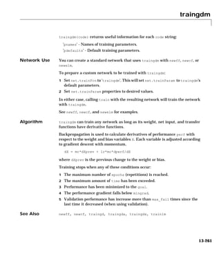
![traingdx
Purpose Gradient descent w/momentum & adaptive lr backpropagation
traingdx
Syntax [net,tr] = traingdx(net,Pd,Tl,Ai,Q,TS,VV)
info = traingdx(code)
Description traingdx is a network training function that updates weight and bias values
according to gradient descent momentum and an adaptive learning rate.
traingdx(net,Pd,Tl,Ai,Q,TS,VV) takes these inputs,
net - Neural network.
Pd - Delayed input vectors.
Tl - Layer target vectors.
Ai - Initial input delay conditions.
Q - Batch size.
TS - Time steps.
VV - Either empty matrix [] or structure of validation vectors.
and returns,
net - Trained network.
TR - Training record of various values over each epoch:
TR.epoch - Epoch number.
TR.perf - Training performance.
TR.vperf - Validation performance.
TR.tperf - Test performance.
TR.lr - Adaptive learning rate.
13-262](https://image.slidesharecdn.com/nnet-090922002848-phpapp01/85/Neural-Network-Toolbox-MATLAB-664-320.jpg)
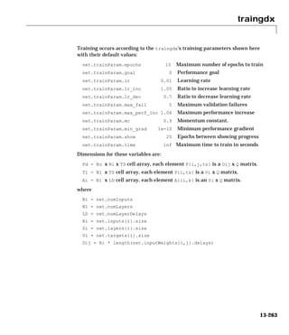
![traingdx
If VV is not [], it must be a structure of validation vectors,
VV.PD - Validation delayed inputs.
VV.Tl - Validation layer targets.
VV.Ai - Validation initial input conditions.
VV.Q - Validation batch size.
VV.TS - Validation time steps.
which is used to stop training early if the network performance on the
validation vectors fails to improve or remains the same for max_fail epochs in
a row.
traingdx(code) return useful information for each code string:
'pnames' - Names of training parameters.
'pdefaults' - Default training parameters.
Network Use You can create a standard network that uses traingdx with newff, newcf, or
newelm.
To prepare a custom network to be trained with traingdx:
1 Set net.trainFcn to 'traingdx'. This will set net.trainParam to traingdx's
default parameters.
2 Set net.trainParam properties to desired values.
In either case, calling train with the resulting network will train the network
with traingdx.
See newff, newcf, and newelm for examples.
Algorithm traingdx can train any network as long as its weight, net input, and transfer
functions have derivative functions.
Backpropagation is used to calculate derivatives of performance perf with
respect to the weight and bias variables X. Each variable is adjusted according
to gradient descent with momentum,
dX = mc*dXprev + lr*mc*dperf/dX
where dXprev is the previous change to the weight or bias.
13-264](https://image.slidesharecdn.com/nnet-090922002848-phpapp01/85/Neural-Network-Toolbox-MATLAB-666-320.jpg)
![trainlm
Purpose Levenberg-Marquardt backpropagation
trainlm
Syntax [net,tr] = trainlm(net,Pd,Tl,Ai,Q,TS,VV)
info = trainlm(code)
Description trainlm is a network training function that updates weight and bias values
according to Levenberg-Marquardt optimization.
trainlm(net,Pd,Tl,Ai,Q,TS,VV) takes these inputs,
net - Neural network.
Pd - Delayed input vectors.
Tl - Layer target vectors.
Ai - Initial input delay conditions.
Q - Batch size.
TS - Time steps.
VV - Either empty matrix [] or structure of validation vectors.
and returns,
net - Trained network.
TR - Training record of various values over each epoch:
TR.epoch - Epoch number.
TR.perf - Training performance.
TR.vperf - Validation performance.
TR.tperf - Test performance.
TR.mu - Adaptive mu value.
13-266](https://image.slidesharecdn.com/nnet-090922002848-phpapp01/85/Neural-Network-Toolbox-MATLAB-668-320.jpg)
![trainlm
Training occurs according to the trainlm's training parameters shown here
with their default values:
net.trainParam.epochs 10 Maximum number of epochs to train
net.trainParam.goal 0 Performance goal
net.trainParam.lr 0.01 Learning rate
net.trainParam.max_fail 5 Maximum validation failures
net.trainParam.mem_reduc 1 Factor to use for memory/speed
trade off
net.trainParam.min_grad 1e-10 Minimum performance gradient
net.trainParam.show 25 Epochs between showing progress
net.trainParam.time inf Maximum time to train in seconds
Dimensions for these variables are:
Pd - No x Ni x TS cell array, each element P{i,j,ts} is a Dij x Q matrix.
Tl - Nl x TS cell array, each element P{i,ts} is a Vi x Q matrix.
Ai - Nl x LD cell array, each element Ai{i,k} is an Si x Q matrix.
where
Ni = net.numInputs
Nl = net.numLayers
LD = net.numLayerDelays
Ri = net.inputs{i}.size
Si = net.layers{i}.size
Vi = net.targets{i}.size
Dij = Ri * length(net.inputWeights{i,j}.delays)
If VV is not [], it must be a structure of validation vectors,
VV.PD - Validation delayed inputs.
VV.Tl - Validation layer targets.
VV.Ai - Validation initial input conditions.
VV.Q - Validation batch size.
VV.TS - Validation time steps.
13-267](https://image.slidesharecdn.com/nnet-090922002848-phpapp01/85/Neural-Network-Toolbox-MATLAB-669-320.jpg)
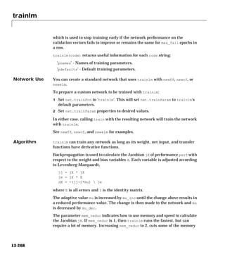
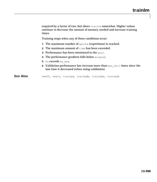
![trainoss
Purpose One step secant backpropagation
trainoss
Syntax [net,tr] = trainoss(net,Pd,Tl,Ai,Q,TS,VV)
info = trainoss(code)
Description trainoss is a network training function that updates weight and bias values
according to the one step secant method.
trainoss(net,Pd,Tl,Ai,Q,TS,VV,TV) takes these inputs,
net - Neural network.
Pd - Delayed input vectors.
Tl - Layer target vectors.
Ai - Initial input delay conditions.
Q - Batch size.
TS - Time steps.
VV - Either empty matrix [] or structure of validation vectors.
TV - Either empty matrix [] or structure of test vectors.
and returns,
net - Trained network.
TR - Training record of various values over each epoch:
TR.epoch - Epoch number.
TR.perf - Training performance.
TR.vperf - Validation performance.
TR.tperf - Test performance.
13-270](https://image.slidesharecdn.com/nnet-090922002848-phpapp01/85/Neural-Network-Toolbox-MATLAB-672-320.jpg)
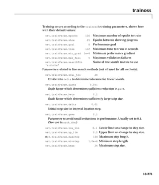
![trainoss
Dimensions for these variables are:
Pd - No x Ni x TS cell array, each element P{i,j,ts} is a Dij x Q matrix.
Tl - Nl x TS cell array, each element P{i,ts} is a Vi x Q matrix.
Ai - Nl x LD cell array, each element Ai{i,k} is an Si x Q matrix.
where
Ni = net.numInputs
Nl = net.numLayers
LD = net.numLayerDelays
Ri = net.inputs{i}.size
Si = net.layers{i}.size
Vi = net.targets{i}.size
Dij = Ri * length(net.inputWeights{i,j}.delays)
If VV is not [], it must be a structure of validation vectors,
VV.PD - Validation delayed inputs.
VV.Tl - Validation layer targets.
VV.Ai - Validation initial input conditions.
VV.Q - Validation batch size.
VV.TS - Validation time steps.
which is used to stop training early if the network performance on the
validation vectors fails to improve or remains the same for max_fail epochs in
a row.
If TV is not [], it must be a structure of validation vectors,
TV.PD - Validation delayed inputs.
TV.Tl - Validation layer targets.
TV.Ai - Validation initial input conditions.
TV.Q - Validation batch size.
TV.TS - Validation time steps.
which is used to test the generalization capability of the trained network.
13-272](https://image.slidesharecdn.com/nnet-090922002848-phpapp01/85/Neural-Network-Toolbox-MATLAB-674-320.jpg)
![trainoss
trainoss(code) returns useful information for each code string:
'pnames' - Names of training parameters.
'pdefaults' - Default training parameters.
Examples Here is a problem consisting of inputs P and targets T that we would like to
solve with a network.
P = [0 1 2 3 4 5];
T = [0 0 0 1 1 1];
Here a two-layer feed-forward network is created. The network's input ranges
from [0 to 10]. The first layer has two tansig neurons, and the second layer
has one logsig neuron. The trainoss network training function is to be used.
Create and Test a Network
net = newff([0 5],[2 1],{'tansig','logsig'},'trainoss');
a = sim(net,p)
Train and Retest the Network
net.trainParam.epochs = 50;
net.trainParam.show = 10;
net.trainParam.goal = 0.1;
net = train(net,p,t);
a = sim(net,p)
See newff, newcf, and newelm for other examples.
Network Use You can create a standard network that uses trainoss with newff, newcf, or
newelm.
To prepare a custom network to be trained with trainoss:
1 Set net.trainFcn to 'trainoss'. This will set net.trainParam to trainoss's
default parameters.
2 Set net.trainParam properties to desired values.
In either case, calling train with the resulting network will train the network
with trainoss.
13-273](https://image.slidesharecdn.com/nnet-090922002848-phpapp01/85/Neural-Network-Toolbox-MATLAB-675-320.jpg)
![trainrp
Purpose RPROP backpropagation
trainrp
Syntax [net,tr] = trainrp(net,Pd,Tl,Ai,Q,TS,VV)
info = trainrp(code)
Description trainrp is a network training function that updates weight and bias values
according to the resilient backpropagation algorithm (RPROP).
trainrp(net,Pd,Tl,Ai,Q,TS,VV,TV) takes these inputs,
net - Neural network.
Pd - Delayed input vectors.
Tl - Layer target vectors.
Ai - Initial input delay conditions.
Q - Batch size.
TS - Time steps.
VV - Either empty matrix [] or structure of validation vectors.
TV - Either empty matrix [] or structure of test vectors.
and returns,
net - Trained network.
TR - Training record of various values over each epoch:
TR.epoch - Epoch number.
TR.perf - Training performance.
TR.vperf - Validation performance.
TR.tperf - Test performance.
13-275](https://image.slidesharecdn.com/nnet-090922002848-phpapp01/85/Neural-Network-Toolbox-MATLAB-677-320.jpg)
![trainrp
If VV is not [], it must be a structure of validation vectors,
VV.PD - Validation delayed inputs.
VV.Tl - Validation layer targets.
VV.Ai - Validation initial input conditions.
VV.Q - Validation batch size.
VV.TS - Validation time steps.
which is used to stop training early if the network performance on the
validation vectors fails to improve or remains the same for max_fail epochs in
a row.
If TV is not [], it must be a structure of validation vectors,
TV.PD - Validation delayed inputs.
TV.Tl - Validation layer targets.
TV.Ai - Validation initial input conditions.
TV.Q - Validation batch size.
TV.TS - Validation time steps.
which is used to test the generalization capability of the trained network.
trainrp(code) returns useful information for each code string:
'pnames' - Names of training parameters.
'pdefaults' - Default training parameters.
Examples Here is a problem consisting of inputs P and targets T that we would like to
solve with a network.
P = [0 1 2 3 4 5];
T = [0 0 0 1 1 1];
Here a two-layer feed-forward network is created. The network's input ranges
from [0 to 10]. The first layer has two tansig neurons, and the second layer
has one logsig neuron. The trainrp network training function is to be used.
Create and Test a Network
net = newff([0 5],[2 1],{'tansig','logsig'},'trainrp');
a = sim(net,p)
13-277](https://image.slidesharecdn.com/nnet-090922002848-phpapp01/85/Neural-Network-Toolbox-MATLAB-679-320.jpg)
![trainscg
Purpose Scaled conjugate gradient backpropagation
trainscg
Syntax [net,tr] = trainscg(net,Pd,Tl,Ai,Q,TS,VV)
info = trainscg(code)
Description trainscg is a network training function that updates weight and bias values
according to the scaled conjugate gradient method.
trainscg(net,Pd,Tl,Ai,Q,TS,VV,TV) takes these inputs,
net - Neural network.
Pd - Delayed input vectors.
Tl - Layer target vectors.
Ai - Initial input delay conditions.
Q - Batch size.
TS - Time steps.
VV - Either empty matrix [] or structure of validation vectors.
TV - Either empty matrix [] or structure of test vectors.
and returns,
net - Trained network.
TR - Training record of various values over each epoch:
TR.epoch - Epoch number.
TR.perf - Training performance.
TR.vperf - Validation performance.
TR.tperf - Test performance.
13-280](https://image.slidesharecdn.com/nnet-090922002848-phpapp01/85/Neural-Network-Toolbox-MATLAB-682-320.jpg)
![trainscg
Training occurs according to the trainscg's training parameters shown here
with their default values:
net.trainParam.epochs 100 Maximum number of epochs to train
net.trainParam.show 25 Epochs between showing progress
net.trainParam.goal 0 Performance goal
net.trainParam.time inf Maximum time to train in seconds
net.trainParam.min_grad 1e-6 Minimum performance gradient
net.trainParam.max_fail 5 Maximum validation failures
net.trainParam.sigma 5.0e-5 Determines change in weight for
second derivative approximation.
net.trainParam.lambda 5.0e-7 Parameter for regulating the
indefiniteness of the Hessian.
Dimensions for these variables are:
Pd - No x Ni x TS cell array, each element P{i,j,ts} is a Dij x Q matrix.
Tl - Nl x TS cell array, each element P{i,ts} is a Vi x Q matrix.
Ai - Nl x LD cell array, each element Ai{i,k} is an Si x Q matrix.
where
Ni = net.numInputs
Nl = net.numLayers
LD = net.numLayerDelays
Ri = net.inputs{i}.size
Si = net.layers{i}.size
Vi = net.targets{i}.size
Dij = Ri * length(net.inputWeights{i,j}.delays)
If VV is not [], it must be a structure of validation vectors,
VV.PD - Validation delayed inputs.
VV.Tl - Validation layer targets.
VV.Ai - Validation initial input conditions.
VV.Q - Validation batch size.
VV.TS - Validation time steps.
13-281](https://image.slidesharecdn.com/nnet-090922002848-phpapp01/85/Neural-Network-Toolbox-MATLAB-683-320.jpg)
![trainscg
which is used to stop training early if the network performance on the
validation vectors fails to improve or remains the same for max_fail epochs in
a row.
If TV is not [], it must be a structure of validation vectors,
TV.PD - Validation delayed inputs.
TV.Tl - Validation layer targets.
TV.Ai - Validation initial input conditions.
TV.Q - Validation batch size.
TV.TS - Validation time steps.
which is used to test the generalization capability of the trained network.
trainscg(code) returns useful information for each code string:
'pnames' - Names of training parameters.
'pdefaults' - Default training parameters.
Examples Here is a problem consisting of inputs P and targets T that we would like to
solve with a network.
P = [0 1 2 3 4 5];
T = [0 0 0 1 1 1];
Here a two-layer feed-forward network is created. The network's input ranges
from [0 to 10]. The first layer has two tansig neurons, and the second layer
has one logsig neuron. The trainscg network training function is to be used.
Create and Test a Network
net = newff([0 5],[2 1],{'tansig','logsig'},'trainscg');
a = sim(net,p)
Train and Retest the Network
net.trainParam.epochs = 50;
net.trainParam.show = 10;
net.trainParam.goal = 0.1;
net = train(net,p,t);
a = sim(net,p)
See newff, newcf, and newelm for other examples.
13-282](https://image.slidesharecdn.com/nnet-090922002848-phpapp01/85/Neural-Network-Toolbox-MATLAB-684-320.jpg)
![trainwb
Purpose By-weight-&-bias 1-vector-at-a-time training function
trainwb
Syntax [net,tr] = trainwb(net,Pd,Tl,Ai,Q,TS,VV)
info = trainwb(code)
Description trainwb is a network training function that updates weight and bias values
according to Levenberg-Marquardt optimization.
trainwb(net,Pd,Tl,Ai,Q,TS,VV) takes these inputs,
net - Neural network.
Pd - Delayed input vectors.
Tl - Layer target vectors.
Ai - Initial input delay conditions.
Q - Batch size.
TS - Time steps.
VV - Either empty matrix [] or structure of validation vectors.
and returns,
net - Trained network.
TR - Training record of various values over each epoch:
TR.epoch - Epoch number.
TR.perf - Training performance.
TR.vperf - Validation performance.
TR.tperf - Test performance.
Training occurs according to the trainwb1's training parameters, shown here
with their default values:
net.trainParam.epochs 100 Maximum number of epochs to train
net.trainParam.goal 0 Performance goal
net.trainParam.max_fail 5 Maximum validation failures
net.trainParam.show 25 Epochs between showing progress
net.trainParam.time inf Maximum time to train in seconds
13-284](https://image.slidesharecdn.com/nnet-090922002848-phpapp01/85/Neural-Network-Toolbox-MATLAB-686-320.jpg)
![trainwb
Dimensions for these variables are:
Pd - No x Ni x TS cell array, each element P{i,j,ts} is a Dij x Q matrix.
Tl - Nl x TS cell array, each element P{i,ts} is a Vi x Q matrix.
Ai - Nl x LD cell array, each element Ai{i,k} is an Si x Q matrix.
where
Ni = net.numInputs
Nl = net.numLayers
LD = net.numLayerDelays
Ri = net.inputs{i}.size
Si = net.layers{i}.size
Vi = net.targets{i}.size
Dij = Ri * length(net.inputWeights{i,j}.delays)
If VV is not [], it must be a structure of validation vectors,
VV.PD - Validation delayed inputs.
VV.Tl - Validation layer targets.
VV.Ai - Validation initial input conditions.
VV.Q - Validation batch size.
VV.TS - Validation time steps.
which is used to stop training early if the network performance on the
validation vectors fails to improve or remains the same for max_fail epochs in
a row.
trainwb(code) returns useful information for each code string:
'pnames' - Names of training parameters.
'pdefaults' - Default training parameters.
Network Use You can create a standard network that uses trainwb with newp or newlin.
13-285](https://image.slidesharecdn.com/nnet-090922002848-phpapp01/85/Neural-Network-Toolbox-MATLAB-687-320.jpg)
![trainwb1
Purpose By-weight-and-bias network training function
trainwb1
Syntax [net,tr] = trainwb1(net,Pd,Tl,Ai,Q,TS,VV)
info = trainwb1(code)
Description trainwb1 is a network training function which updates each weight and bias
according to its learning function. At each epoch trainwb1 randomly chooses
just one input vector (or sequence) to present to the network.
trainwb1(net,Pd,Tl,Ai,Q,TS,VV) takes these inputs,
net - Neural network.
Pd - Delayed input vectors.
Tl - Layer target vectors.
Ai - Initial input delay conditions.
Q - Batch size.
TS - Time steps.
VV - Either empty matrix [] or structure of validation vectors.
and returns,
net - Trained network.
TR - Training record of various values over each epoch:
TR.epoch - Epoch number.
TR.perf - Training performance.
TR.index - Index of presented input vector (or sequence).
Training occurs according to the trainwb1's training parameters shown here
with their default values:
net.trainParam.epochs 100 Maximum number of epochs to train
net.trainParam.show 25 Epochs between showing progress
net.trainParam.time inf Maximum time to train in seconds
13-287](https://image.slidesharecdn.com/nnet-090922002848-phpapp01/85/Neural-Network-Toolbox-MATLAB-689-320.jpg)
![tramnmx
Purpose Transform data using a precalculated min and max
tramnmx
Syntax [pn] = tramnmx(p,minp,maxp)
Description tramnmx transforms the network input set using minimum and maximum
values that were previously computed by premnmx. This function needs to be
used when a network has been trained using data normalized by premnmx. All
subsequent inputs to the network need to be transformed using the same
normalization.
tramnmx(P,minp, maxp)takes these inputs
P - R x Q matrix of input (column) vectors.
minp- R x 1 vector containing original minimums for each input.
maxp- R x 1 vector containing original maximums for each input.
and returns,
PN - R x Q matrix of normalized input vectors
Examples Here is the code to normalize a given data set, so that the inputs and targets
will fall in the range [-1,1], using premnmx, and also code to train a network
with the normalized data.
p = [-10 -7.5 -5 -2.5 0 2.5 5 7.5 10];
t = [0 7.07 -10 -7.07 0 7.07 10 7.07 0];
[pn,minp,maxp,tn,mint,maxt] = premnmx(p,t);
net = newff(minmax(pn),[5 1],{'tansig' 'purelin'},'trainlm');
net = train(net,pn,tn);
If we then receive new inputs to apply to the trained network, we will use
tramnmx to transform them first. Then the transformed inputs can be used to
simulate the previously trained network. The network output must also be
unnormalized using postmnmx.
p2 = [4 -7];
[p2n] = tramnmx(p2,minp,maxp);
an = sim(net,pn);
[a] = postmnmx(an,mint,maxt);
Algorithm pn = 2*(p-minp)/(maxp-minp) - 1;
See Also premnmx, prestd, prepca, trastd, trapca
13-290](https://image.slidesharecdn.com/nnet-090922002848-phpapp01/85/Neural-Network-Toolbox-MATLAB-692-320.jpg)
![trapca
Purpose Principal component transformation
trapca
Syntax [Ptrans] = trapca(P,TransMat)
Description trapca preprocesses the network input training set by applying the principal
component transformation that was previously computed by prepca. This
function needs to be used when a network has been trained using data
normalized by prepca. All subsequent inputs to the network need to be
transformed using the same normalization.
trapca(P,TransMat) takes these inputs,
P - R x Q matrix of centered input (column) vectors.
TransMat - Transformation matrix.
and returns,
Ptrans - Transformed data set.
Examples Here is the code to perform a principal component analysis and retain only
those components which contribute more than 2 percent to the variance in the
data set. prestd is called first to create zero mean data, which are needed for
prepca.
p = [-1.5 -0.58 0.21 -0.96 -0.79; -2.2 -0.87 0.31 -1.4 -1.2];
t = [-0.08 3.4 -0.82 0.69 3.1];
[pn,meanp,stdp,tn,meant,stdt] = prestd(p,t);
[ptrans,transMat] = prepca(pn,0.02);
net = newff(minmax(ptrans),[5 1],{'tansig''purelin'},'trainlm');
net = train(net,ptrans,tn);
If we then receive new inputs to apply to the trained network, we will use
trastd and trapca to transform them first. Then the transformed inputs can
be used to simulate the previously trained network. The network output must
also be unnormalized using poststd.
p2 = [1.5 -0.8;0.05 -0.3];
[p2n] = trastd(p2,meanp,stdp);
[p2trans] = trapca(p2n,TransMat)
an = sim(net,p2trans);
[a] = poststd(an,meant,stdt);
13-291](https://image.slidesharecdn.com/nnet-090922002848-phpapp01/85/Neural-Network-Toolbox-MATLAB-693-320.jpg)

![trastd
Purpose Preprocess data using a precalculated mean and standard deviation
trastd
Syntax [pn] = trastd(p,meanp,stdp)
Description trastd preprocesses the network training set using the mean and standard
deviation that were previously computed by prestd. This function needs to be
used when a network has been trained using data normalized by prestd. All
subsequent inputs to the network need to be transformed using the same
normalization.
trastd(P,T) takes these inputs,
P - R x Q matrix of input (column) vectors.
meanp - R x 1 vector containing the original means for each input.
stdp - R x 1 vector containing the original standard deviations for each
input.
and returns,
PN - R x Q matrix of normalized input vectors.
Examples Here is the code to normalize a given data set so that the inputs and targets
will have means of zero and standard deviations of 1.
p = [-0.92 0.73 -0.47 0.74 0.29; -0.08 0.86 -0.67 -0.52 0.93];
t = [-0.08 3.4 -0.82 0.69 3.1];
[pn,meanp,stdp,tn,meant,stdt] = prestd(p,t);
net = newff(minmax(pn),[5 1],{'tansig' 'purelin'},'trainlm');
net = train(net,pn,tn);
If we then receive new inputs to apply to the trained network, we will use
trastd to transform them first. Then the transformed inputs can be used to
simulate the previously trained network. The network output must also be
unnormalized using poststd.
p2 = [1.5 -0.8;0.05 -0.3];
[p2n] = trastd(p2,meanp,stdp);
an = sim(net,pn);
[a] = poststd(an,meant,stdt);
Algorithm pn = (p-meanp)/stdp;
See Also premnmx, prepca, prestd, trapca, tramnmx
13-293](https://image.slidesharecdn.com/nnet-090922002848-phpapp01/85/Neural-Network-Toolbox-MATLAB-695-320.jpg)
![vec2ind
Purpose Convert vectors to indices
vec2ind
Syntax ind = vec2ind(vec)
Description ind2vec and vec2ind allow indices to be represented either by themselves or as
vectors containing a 1 in the row of the index they represent.
vec2ind(vec) takes one argument,
vec - Matrix of vectors, each containing a single 1.
and returns the indices of the 1's.
Examples Here four vectors (containing only one 1 each) are defined and the indices of the
1's are found.
vec = [1 0 0 0; 0 0 1 0; 0 1 0 1]
ind = vec2ind(vec)
See Also ind2vec
13-295](https://image.slidesharecdn.com/nnet-090922002848-phpapp01/85/Neural-Network-Toolbox-MATLAB-697-320.jpg)


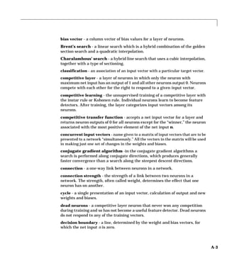
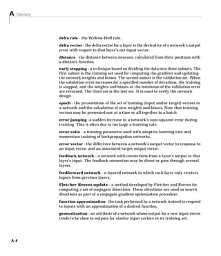


![Mathematical Notation for Equations and Figures
k, l
Input Weight Matrix IW
k, l
Layer Weight Matrix LW
Figure and Equation Examples
The following figure, taken from Chapter 11, “Advanced Topics,” illustrates
notation used in such advanced figures.
Inputs Layers 1 and 2 Layer 3 Outputs
p1(k)
IW1,1
2x1 TDL
n1(k) 1 LW3,3
4x2
4x1 1 x (1*1)
1 b1 a1(k)
4x1
IW3,1
2 4x1 4 1x4
n3(k) a3(k) y2(k)
1x1 1x1 1x1
a1(k) = tansig (IW1,1p1(k) +b1) 1 b3
1x1
a2(k) 1
TDL IW 2,1
LW3,2
0,1 3x1
n2(k) 1x3 y1(k)
3 x (2*2)
3x1 3x1
p2(k)
TDL IW2,2
5x1 1
5 3 x (1*5) 3
a2(k) = logsig (IW2,1 [p1(k);p1(k-1) ]+ IW2,2p2(k-1)) a3(k)=purelin(LW3,3a3(k-1)+IW3,1 a1 (k)+b3+LW3,2a2 (k))
B-3](https://image.slidesharecdn.com/nnet-090922002848-phpapp01/85/Neural-Network-Toolbox-MATLAB-713-320.jpg)

![C Bibliography
[Batt92] Battiti, R., “First and second order methods for learning: Between
steepest descent and Newton’s method,” Neural Computation, vol. 4, no. 2, pp.
141–166, 1992.
[Beal72] Beale, E. M. L., “A derivation of conjugate gradients,” in F. A.
Lootsma, ed., Numerical methods for nonlinear optimization, London:
Academic Press, 1972.
[Bren73] Brent, R. P., Algorithms for Minimization Without Derivatives,
Englewood Cliffs, NJ: Prentice-Hall, 1973.
[Caud89] Caudill, M., Neural Networks Primer, San Francisco, CA: Miller
Freeman Publications, 1989.
This collection of papers from the AI Expert Magazine gives an excellent
introduction to the field of neural networks. The papers use a minimum of
mathematics to explain the main results clearly. Several good suggestions for
further reading are included.
[CaBu92] Caudill, M., and C. Butler, Understanding Neural Networks:
Computer Explorations, Vols. 1 and 2, Cambridge, MA: the MIT Press, 1992.
This is a two volume workbook designed to give students “hands on” experience
with neural networks. It is written for a laboratory course at the senior or
first-year graduate level. Software for IBM PC and Apple Macintosh computers
is included. The material is well written, clear and helpful in understanding a
field that traditionally has been buried in mathematics.
[Char92] Charalambous, C.,“Conjugate gradient algorithm for efficient
training of artificial neural networks,” IEEE Proceedings, vol. 139, no. 3, pp.
301–310, 1992.
[ChCo91] Chen, S., C. F. N. Cowan, and P. M. Grant, “Orthogonal least
squares learning algorithm for radial basis function networks,” IEEE
Transactions on Neural Networks, vol. 2, no. 2, pp. 302-309, 1991.
This paper gives an excellent introduction to the field of radial basis functions.
The papers use a minimum of mathematics to explain the main results clearly.
Several good suggestions for further reading are included.
[DARP88] DARPA Neural Network Study, Lexington, MA: M.I.T. Lincoln
Laboratory, 1988.
This book is a compendium of knowledge of neural networks as they were
known to 1988. It presents the theoretical foundations of neural networks and
C-2](https://image.slidesharecdn.com/nnet-090922002848-phpapp01/85/Neural-Network-Toolbox-MATLAB-716-320.jpg)
![discusses their current applications. It contains sections on associative
memories, recurrent networks, vision, speech recognition, and robotics.
Finally, it discusses simulation tools and implementation technology.
[DeSc83] Dennis, J. E., and R. B. Schnabel, Numerical Methods for
Unconstrained Optimization and Nonlinear Equations, Englewood Cliffs, NJ:
Prentice-Hall, 1983.
[Elma90] Elman, J. L.,“Finding structure in time,” Cognitive Science, vol. 14,
pp. 179-211, 1990.
This paper is a superb introduction to the Elman networks described in
Chapter 10, “Recurrent Networks.”
[FlRe64] Fletcher, R., and C. M. Reeves, “Function minimization by conjugate
gradients,” Computer Journal, vol. 7, pp. 149-154, 1964.
[FoHa97] Foresee, F. D., and M. T. Hagan, “Gauss-Newton approximation to
Bayesian regularization,” Proceedings of the 1997 International Joint
Conference on Neural Networks,, pages 1930-1935, 1997.
[GiMu81] Gill, P. E., W. Murray, and M. H. Wright, Practical Optimization,
New York: Academic Press, 1981.
[Gros82] Grossberg, S., Studies of the Mind and Brain, Drodrecht, Holland:
Reidel Press, 1982.
This book contains articles summarizing Grossberg’s theoretical
psychophysiology work up to 1980. Each article contains a preface explaining
the main points.
[HaMe94] Hagan, M. T., and M. Menhaj, “Training feedforward networks with
the Marquardt algorithm,” IEEE Transactions on Neural Networks, vol. 5, no. 6, pp.
989–993, 1994.
This paper reports the first development of the Levenberg-Marquardt
algorithm for neural networks. It describes the theory and application of the
algorithm, which trains neural networks at a rate 10 to 100 times faster than
the usual gradient descent backpropagation method.
[HDB96] Hagan, M. T., H. B. Demuth, and M. H. Beale, Neural Network
Design, Boston, MA: PWS Publishing, 1996.
[Hebb49] Hebb, D. O., The Organization of Behavior, New York: Wiley, 1949.
C-3](https://image.slidesharecdn.com/nnet-090922002848-phpapp01/85/Neural-Network-Toolbox-MATLAB-717-320.jpg)
![C Bibliography
This book proposed neural network architectures and the first learning rule.
The learning rule is used to form a theory of how collections of cells might form
a concept.
[Himm72] Himmelblau, D. M., Applied Nonlinear Programming, New York:
McGraw-Hill, 1972.
[Joll86] Jolliffe, I. T., Principal Component Analysis, New York:
Springer-Verlag, 1986.
[Koho87] Kohonen, T., Self-Organization and Associative Memory, 2nd
Edition, Berlin: Springer-Verlag, 1987.
This book analyzes several learning rules. The Kohonen learning rule is then
introduced and embedded in self-organizing feature maps. Associative
networks are also studied.
[LiMi89] Li, J., A. N. Michel, and W. Porod, “Analysis and synthesis of a class
of neural networks: linear systems operating on a closed hypercube,” IEEE
Transactions on Circuits and Systems, vol. 36, no. 11, pp. 1405-1422, 1989.
This paper discusses a class of neural networks described by first order linear
differential equations that are defined on a closed hypercube. The systems
considered retain the basic structure of the Hopfield model but are easier to
analyze and implement. The paper presents an efficient method for
determining the set of asymptotically stable equilibrium points and the set of
unstable equilibrium points. Examples are presented. The method of Li et. al.
is implemented in Chapter 9 of this Users Guide.
[Lipp87] Lippman, R. P., “An introduction to computing with neural nets,”
IEEE ASSP Magazine, pp. 4-22, 1987.
This paper gives an introduction to the field of neural nets by reviewing six
neural net models that can be used for pattern classification.The paper shows
how existing classification and clustering algorithms can be performed using
simple components that are like neurons. This is a highly readable paper.
[MacK92] MacKay, D. J. C., “Bayesian interpolation,” Neural Computation,
vol. 4, no. 3, pp. 415-447, 1992.
[McPi43] McCulloch, W. S., and W. H. Pitts, “A logical calculus of ideas
immanent in nervous activity,” Bulletin of Mathematical Biophysics, vol. 5, pp.
115-133, 1943.
C-4](https://image.slidesharecdn.com/nnet-090922002848-phpapp01/85/Neural-Network-Toolbox-MATLAB-718-320.jpg)
![A classic paper that describes a model of a neuron that is binary and has a fixed
threshold. A network of such neurons can perform logical operations.
[Moll93] Moller, M. F., “A scaled conjugate gradient algorithm for fast
supervised learning,” Neural Networks, vol. 6, pp. 525-533, 1993.
[NgWi89] Nguyen, D., and B. Widrow, “The truck backer-upper: An example
of self-learning in neural networks,” Proceedings of the International Joint
Conference on Neural Networks, vol 2, pp. 357-363, 1989.
This paper describes a two-layer network that first learned the truck dynamics
and then learned how to back the truck to a specified position at a loading dock.
To do this, the neural network had to solve a highly nonlinear control systems
problem.
[NgWi90] Nguyen, D., and B. Widrow, “Improving the learning speed of
2-layer neural networks by choosing initial values of the adaptive weights,”
Proceedings of the International Joint Conference on Neural Networks, vol 3,
pp. 21-26, 1990.
Nguyen and Widrow demonstrate that a 2-layer sigmoid/linear network can be
viewed as performing a piecewise linear approximation of any learned
function. It is shown that weights and biases generated with certain
constraints will result in an initial network better able to form a function
approximation of an arbitrary function. Use of the Nguyen-Widrow (instead of
purely random) initial conditions often shortens training time by more than an
order of magnitude.
[Powe77] Powell, M. J. D., “Restart procedures for the conjugate gradient
method,” Mathematical Programming, vol. 12, pp. 241-254, 1977.
[Pulu92] N. Purdie, E.A. Lucas and M.B. Talley, "Direct measure of total
cholesterol and its distribution among major serum lipoproteins," Clinical
Chemistry, vol. 38, no. 9, pp. 1645-1647, 1992.
[RiBr93] Riedmiller, M., and H. Braun, “A direct adaptive method for faster
backpropagation learning: The RPROP algorithm,” Proceedings of the IEEE
International Conference on Neural Networks, 1993.
[Rose61] Rosenblatt, F., Principles of Neurodynamics, Washington D.C.:
Spartan Press, 1961.
This book presents all of Rosenblatt’s results on perceptrons. In particular, it
presents his most important result, the perceptron learning theorem.
C-5](https://image.slidesharecdn.com/nnet-090922002848-phpapp01/85/Neural-Network-Toolbox-MATLAB-719-320.jpg)
![C Bibliography
[RuHi86a] Rumelhart, D. E., G. E. Hinton, and R. J. Williams, “Learning
internal representations by error propagation,”, in D. E. Rumelhart and J. L.
McClelland, eds. Parallel Data Processing, vol.1, Cambridge, MA: The M.I.T.
Press, pp. 318-362, 1986.
This is a basic reference on backpropagation.
[RuHi86b] Rumelhart, D. E., G. E. Hinton, and R. J. Williams, “Learning
representations by back-propagating errors,” Nature, vol. 323, pp. 533–536,
1986.
[RuMc86] Rumelhart, D. E., J. L. McClelland, and the PDP Research Group,
eds., Parallel Distributed Processing, Vols. 1 and 2, Cambridge, MA: The M.I.T.
Press, 1986.
These two volumes contain a set of monographs that present a technical
introduction to the field of neural networks. Each section is written by different
authors. These works present a summary of most of the research in neural
networks to the date of publication.
[Scal85] Scales, L. E., Introduction to Non-Linear Optimization, New York:
Springer-Verlag, 1985.
[VoMa88] Vogl, T. P., J. K. Mangis, A. K. Rigler, W. T. Zink, and D. L. Alkon,
“Accelerating the convergence of the backpropagation method,” Biological
Cybernetics, vol. 59, pp. 256-264, 1988.
Backpropagation learning can be speeded up and made less sensitive to small
features in the error surface such as shallow local minima by combining
techniques such as batching, adaptive learning rate, and momentum.
[Wass93] Wasserman, P. D., Advanced Methods in Neural Computing, New
York: Van Nostrand Reinhold, 1993.
[WiHo60] Widrow, B., and M. E. Hoff, “Adaptive switching circuits,” 1960 IRE
WESCON Convention Record, New York IRE, pp. 96-104, 1960.
[WiSt85] Widrow, B., and S. D. Sterns, Adaptive Signal Processing, New York:
Prentice-Hall, 1985.
This is a basic paper on adaptive signal processing.
C-6](https://image.slidesharecdn.com/nnet-090922002848-phpapp01/85/Neural-Network-Toolbox-MATLAB-720-320.jpg)

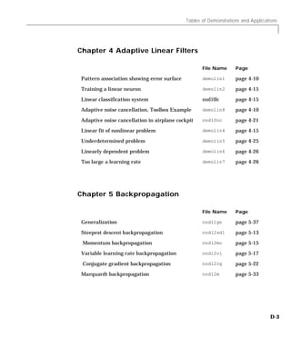
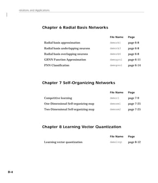

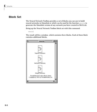
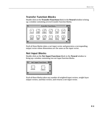
![Block Generation
Block Generation
The function gensim generates block descriptions of networks so you can
simulate them in Simulink.
gensim(net,st)
The second argument to gensim determines the sample time, which is normally
chosen to be some positive real value.
If a network has no delays associated with its input weights or layer weights
this value can be set to -1. A value of -1 tells gensim to generate a network with
continuous sampling.
Example
Here is a simple problem defining a set of inputs p and corresponding targets t:
p = [1 2 3 4 5];
t = [1 3 5 7 9];
The code below designs a linear layer to solve this problem.
net = newlind(p,t)
We can test the network on our original inputs with sim.
y = sim(net,p)
The results returned show the network has solved the problem.
y =
1.0000 3.0000 5.0000 7.0000 9.0000
Call gensim as follows to generate a Simulink version of the network:
gensim(net,-1)
The second argument is -1 so the resulting network block will sample
continuously.
The call to gensim results in the following screen appearing. It contains a
Simulink system consisting of the linear network connected to a sample input
and a scope.
E-5](https://image.slidesharecdn.com/nnet-090922002848-phpapp01/85/Neural-Network-Toolbox-MATLAB-731-320.jpg)
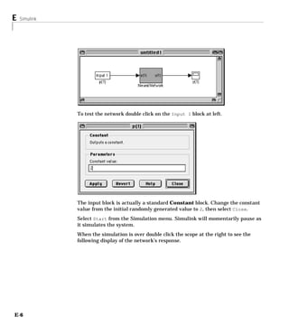


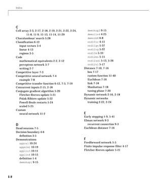
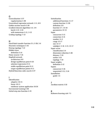

This document is a user's guide for version 3.0 of the Neural Network Toolbox. It introduces neural networks and their applications. Key features of version 3.0 include a reduced memory Levenberg-Marquardt training algorithm, new network types like probabilistic neural networks and generalized regression networks, modular network representations, improved Simulink support, and general toolbox improvements. The guide provides basic information on neural network concepts and architectures.