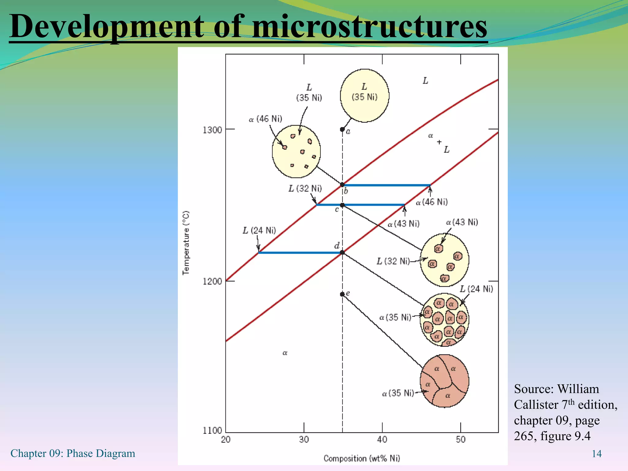
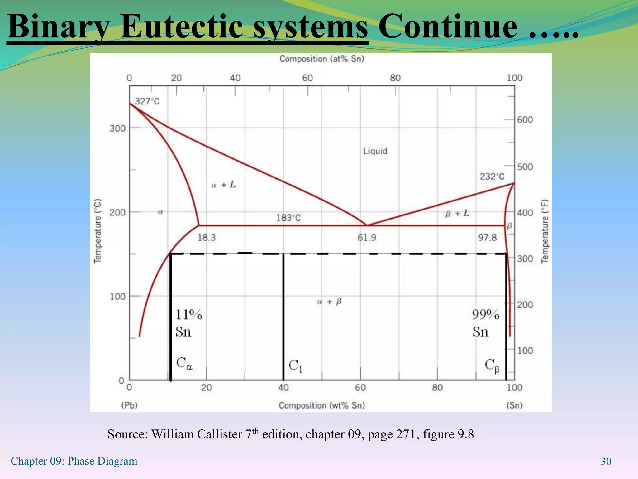
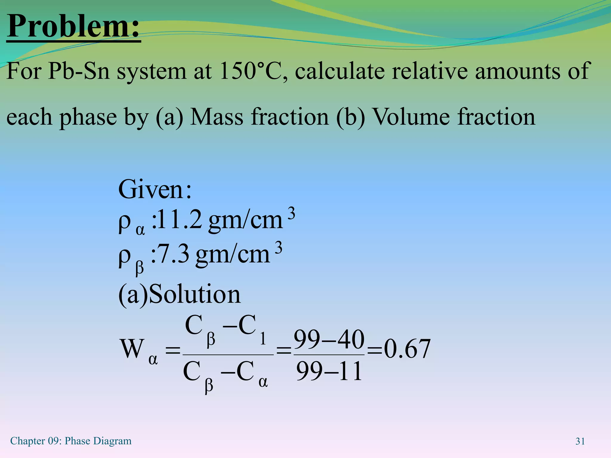
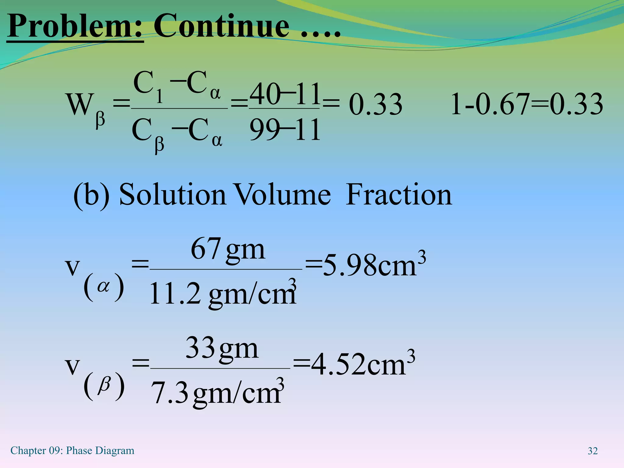
1
Chapter 09: Phase Diagram 2
Introduction
Phase Diagrams are road maps
Chapter 09: Phase Diagram 3
Component: Pure metals/compounds of which an alloy is
composed
System: Alloy system, e.g., Iron-Carbon alloy system,
copper-nickel alloy system
Solid solutions
- Substitutional
- Interstitial
Chapter 09: Phase Diagram 4
Solubility Limit: Max concentration of solute atoms that
may dissolve in the solvent to form a solid solution.
Phases: Homogenous portion of a system that has uniform
physical and chemical properties
Chapter 09: Phase Diagram 5
Source: William Callister 7th edition, chapter 09, page 254, figure 9.1
Chapter 09: Phase Diagram 6
Each phase has different phase physical properties
Microstructure
•Characterized by number of phases, proportions and the
manner of distribution of phases.
•Depends on: Alloying elements, concentrations, heat
treatment (temp, heating/cooling rate etc.)
Chapter 09: Phase Diagram 7
Phase equilibria
Free energy
Equilibrium
Phase equilibrium
Non-equilibrium state: State of equilibrium is never
reached since the rate of approach to equilibrium is very
slow.
Chapter 09: Phase Diagram 8
Equilibrium phase diagram
•Represents the relationships between temperature and
compositions, and the quantities of phases in equilibrium
•Binary Alloy: two components
Chapter 09: Phase Diagram 9
Binary Isomorphous Systems
Source: William Callister 7th edition, chapter 09, page 259, figure 9.3 a&b
Chapter 09: Phase Diagram 10
Isomorphous: Complete solubility in both liquid and solid
states
Three kinds of info:
•Phases,
•compositions,
•percentages/fractions of phases
Chapter 09: Phase Diagram 11
73%
0.73
32
43
35
43
WL





27%
0.27
32
43
32
35
W 





Where, WL: weight fraction of liquid
At 1250°C and Co=35% Ni
Chapter 09: Phase Diagram 12
Inverse lever rule
1.Draw tie-line across the two phase region
2.Locate the overall composition (e.g., Co=35%Ni)
3.To compute the fraction of one phase, take the length of
the tie-line from the overall composition to the opposite
phase boundary and divide by the total tie line length
4.Repeat above procedure for the other phase.
Chapter 09: Phase Diagram 13
------------------ (1)
------------------ (2)
Where, Cs and C both are same
Chapter 09: Phase Diagram 14
Development of microstructures
Source: William
Callister 7th edition,
chapter 09, page
265, figure 9.4
Chapter 09: Phase Diagram 15
Source: William
Callister 7th edition,
chapter 09, page 267,
figure 9.5
Development of microstructures
continue…
Chapter 09: Phase Diagram 16
Development of Microstructures
The compositions readjust with changes in temperature.
These changes occur through the process of diffusion.
Because diffusion is time-dependent, much more time is
required, at each temperature for compositional
adjustments. Diffusion rates decrease with temperature. In
reality, cooling rates are so fast that there is little time to
enable equilibrium cooling.
Chapter 09: Phase Diagram 17
•Because of fast cooling, there is a
non-uniform distribution of the two
elements for isomorphous alloys
“Segregation”
In the centre of each grain, the high
melting element solidifies first. At the
periphery, the low melting element
solidifies.
Non-Equilibrium Solidification
Chapter 09: Phase Diagram 18
Coring
Cored Structure: Concentration contours
•Undesirable less than optimal properties due to
inhomogeneity.
•Coring is eliminated by a homogenization treatment. At a
temperature below the solidus point for the composition;
atomic diffusion causes homogenization.
Chapter 09: Phase Diagram 19
Mechanical Properties of Isomorphous
Alloys
Source: William Callister 7th edition, chapter 09, page 268, figure 9.6
Chapter 09: Phase Diagram 20
•Solid solution hardening or an increase in strength and
hardness by the addition of the other component
•At an intermediate composition, the curve (TS Vs Comp)
passes through a maximum
Mechanical Properties of Isomorphous
Alloys
Chapter 09: Phase Diagram 21
Binary eutectic systems
Source: William Callister 7th edition, chapter 09, page 269, figure 9.7
Chapter 09: Phase Diagram 22
Binary eutectic systems Continue …..
:Solid Solution of Ag in Cu-Rich solvent
:Solid solution of Cu in Ag-Rich solvent
Technically, : Pure Cu
: Pure Ag
Below BEG, only limited solid solubility takes place
Chapter 09: Phase Diagram 23
CEA: (solid) solubility limit for Ag in – phase (Cu-Rich)
HGF: Solubility limit for Cu in -phase (Ag-Rich)
CBA is between /(+) and /(+L) phase regions
•Max. at 7.9% Ag (780°C)
Binary eutectic systems Continue …..
•Decrease to zero at 1085°C (Melting point of pure Cu)
Chapter 09: Phase Diagram 24
For –phase CB: solvus line: /(+)
AB: Solidus line: /(+L)
Binary eutectic systems Continue …..
Chapter 09: Phase Diagram 25
Prepare similar notes for -phase region
HGF is between
For -phase
HG: Solvus line and GF: Solidus line
Binary eutectic systems Continue …..
Chapter 09: Phase Diagram 26
Three two-phase regions: +L, +L and +
E: Eutectic invariant point
CE: 71.9 wt% Ag
Cu-Ag system: TE: 780°C
Binary eutectic systems Continue …..
Chapter 09: Phase Diagram 27
Binary Eutectic systems Continue …..
Eutectic Reaction:
Liquid Solid 1 + Solid 2
L  + 
L(CE)  (C E) +  (C E)
At E,
Chapter 09: Phase Diagram 28
Binary Eutectic systems Continue …..
For Cu-Ag system,
L(71.9 wt% Ag)  (7.9 wt% Ag) +
 (91.2 wt% Ag)
Chapter 09: Phase Diagram 29
Binary Eutectic systems Continue …..
Solidus line at 780°C: Eutectic isotherm
Phase volume fractions represent proportions seen in the
microstructure; so they can be estimated from
microstructures, and the mechanical properties can be
estimated as well.
Chapter 09: Phase Diagram 30
Source: William Callister 7th edition, chapter 09, page 271, figure 9.8
Binary Eutectic systems Continue …..
Chapter 09: Phase Diagram 31
Problem:
For Pb-Sn system at 150°C, calculate relative amounts of
each phase by (a) Mass fraction (b) Volume fraction
0.67
11
99
40
99
C
C
C
C
W
n
(a)Solutio
gm/cm
7.3
:
ρ
gm/cm
11.2
:
ρ
:
Given
α
β
1
β
α
3
β
3
α







Chapter 09: Phase Diagram 32
Problem: Continue ….
3
3
3
3
α
β
α
1
β
cm
4.52
gm/cm
7.3
gm
33
)
(
v
cm
5.98
gm/cm
11.2
gm
67
)
(
v
Fraction
Volume
(b) Solution
0.33
11
99
11
40
C
C
C
C
W













1-0.67=0.33
Chapter 09: Phase Diagram 33
0.43
4.52
5.98
4.52
v
v
v
V
0.57
4.52
5.98
5.98
v
v
v
V
Fraction
Volume
β
α
β
β
β
α
α
α










Problem: Continue ….

Phase diagrams.ppt

  • 1.
  • 2.
    Chapter 09: PhaseDiagram 2 Introduction Phase Diagrams are road maps
  • 3.
    Chapter 09: PhaseDiagram 3 Component: Pure metals/compounds of which an alloy is composed System: Alloy system, e.g., Iron-Carbon alloy system, copper-nickel alloy system Solid solutions - Substitutional - Interstitial
  • 4.
    Chapter 09: PhaseDiagram 4 Solubility Limit: Max concentration of solute atoms that may dissolve in the solvent to form a solid solution. Phases: Homogenous portion of a system that has uniform physical and chemical properties
  • 5.
    Chapter 09: PhaseDiagram 5 Source: William Callister 7th edition, chapter 09, page 254, figure 9.1
  • 6.
    Chapter 09: PhaseDiagram 6 Each phase has different phase physical properties Microstructure •Characterized by number of phases, proportions and the manner of distribution of phases. •Depends on: Alloying elements, concentrations, heat treatment (temp, heating/cooling rate etc.)
  • 7.
    Chapter 09: PhaseDiagram 7 Phase equilibria Free energy Equilibrium Phase equilibrium Non-equilibrium state: State of equilibrium is never reached since the rate of approach to equilibrium is very slow.
  • 8.
    Chapter 09: PhaseDiagram 8 Equilibrium phase diagram •Represents the relationships between temperature and compositions, and the quantities of phases in equilibrium •Binary Alloy: two components
  • 9.
    Chapter 09: PhaseDiagram 9 Binary Isomorphous Systems Source: William Callister 7th edition, chapter 09, page 259, figure 9.3 a&b
  • 10.
    Chapter 09: PhaseDiagram 10 Isomorphous: Complete solubility in both liquid and solid states Three kinds of info: •Phases, •compositions, •percentages/fractions of phases
  • 11.
    Chapter 09: PhaseDiagram 11 73% 0.73 32 43 35 43 WL      27% 0.27 32 43 32 35 W       Where, WL: weight fraction of liquid At 1250°C and Co=35% Ni
  • 12.
    Chapter 09: PhaseDiagram 12 Inverse lever rule 1.Draw tie-line across the two phase region 2.Locate the overall composition (e.g., Co=35%Ni) 3.To compute the fraction of one phase, take the length of the tie-line from the overall composition to the opposite phase boundary and divide by the total tie line length 4.Repeat above procedure for the other phase.
  • 13.
    Chapter 09: PhaseDiagram 13 ------------------ (1) ------------------ (2) Where, Cs and C both are same
  • 14.
    Chapter 09: PhaseDiagram 14 Development of microstructures Source: William Callister 7th edition, chapter 09, page 265, figure 9.4
  • 15.
    Chapter 09: PhaseDiagram 15 Source: William Callister 7th edition, chapter 09, page 267, figure 9.5 Development of microstructures continue…
  • 16.
    Chapter 09: PhaseDiagram 16 Development of Microstructures The compositions readjust with changes in temperature. These changes occur through the process of diffusion. Because diffusion is time-dependent, much more time is required, at each temperature for compositional adjustments. Diffusion rates decrease with temperature. In reality, cooling rates are so fast that there is little time to enable equilibrium cooling.
  • 17.
    Chapter 09: PhaseDiagram 17 •Because of fast cooling, there is a non-uniform distribution of the two elements for isomorphous alloys “Segregation” In the centre of each grain, the high melting element solidifies first. At the periphery, the low melting element solidifies. Non-Equilibrium Solidification
  • 18.
    Chapter 09: PhaseDiagram 18 Coring Cored Structure: Concentration contours •Undesirable less than optimal properties due to inhomogeneity. •Coring is eliminated by a homogenization treatment. At a temperature below the solidus point for the composition; atomic diffusion causes homogenization.
  • 19.
    Chapter 09: PhaseDiagram 19 Mechanical Properties of Isomorphous Alloys Source: William Callister 7th edition, chapter 09, page 268, figure 9.6
  • 20.
    Chapter 09: PhaseDiagram 20 •Solid solution hardening or an increase in strength and hardness by the addition of the other component •At an intermediate composition, the curve (TS Vs Comp) passes through a maximum Mechanical Properties of Isomorphous Alloys
  • 21.
    Chapter 09: PhaseDiagram 21 Binary eutectic systems Source: William Callister 7th edition, chapter 09, page 269, figure 9.7
  • 22.
    Chapter 09: PhaseDiagram 22 Binary eutectic systems Continue ….. :Solid Solution of Ag in Cu-Rich solvent :Solid solution of Cu in Ag-Rich solvent Technically, : Pure Cu : Pure Ag Below BEG, only limited solid solubility takes place
  • 23.
    Chapter 09: PhaseDiagram 23 CEA: (solid) solubility limit for Ag in – phase (Cu-Rich) HGF: Solubility limit for Cu in -phase (Ag-Rich) CBA is between /(+) and /(+L) phase regions •Max. at 7.9% Ag (780°C) Binary eutectic systems Continue ….. •Decrease to zero at 1085°C (Melting point of pure Cu)
  • 24.
    Chapter 09: PhaseDiagram 24 For –phase CB: solvus line: /(+) AB: Solidus line: /(+L) Binary eutectic systems Continue …..
  • 25.
    Chapter 09: PhaseDiagram 25 Prepare similar notes for -phase region HGF is between For -phase HG: Solvus line and GF: Solidus line Binary eutectic systems Continue …..
  • 26.
    Chapter 09: PhaseDiagram 26 Three two-phase regions: +L, +L and + E: Eutectic invariant point CE: 71.9 wt% Ag Cu-Ag system: TE: 780°C Binary eutectic systems Continue …..
  • 27.
    Chapter 09: PhaseDiagram 27 Binary Eutectic systems Continue ….. Eutectic Reaction: Liquid Solid 1 + Solid 2 L  +  L(CE)  (C E) +  (C E) At E,
  • 28.
    Chapter 09: PhaseDiagram 28 Binary Eutectic systems Continue ….. For Cu-Ag system, L(71.9 wt% Ag)  (7.9 wt% Ag) +  (91.2 wt% Ag)
  • 29.
    Chapter 09: PhaseDiagram 29 Binary Eutectic systems Continue ….. Solidus line at 780°C: Eutectic isotherm Phase volume fractions represent proportions seen in the microstructure; so they can be estimated from microstructures, and the mechanical properties can be estimated as well.
  • 30.
    Chapter 09: PhaseDiagram 30 Source: William Callister 7th edition, chapter 09, page 271, figure 9.8 Binary Eutectic systems Continue …..
  • 31.
    Chapter 09: PhaseDiagram 31 Problem: For Pb-Sn system at 150°C, calculate relative amounts of each phase by (a) Mass fraction (b) Volume fraction 0.67 11 99 40 99 C C C C W n (a)Solutio gm/cm 7.3 : ρ gm/cm 11.2 : ρ : Given α β 1 β α 3 β 3 α       
  • 32.
    Chapter 09: PhaseDiagram 32 Problem: Continue …. 3 3 3 3 α β α 1 β cm 4.52 gm/cm 7.3 gm 33 ) ( v cm 5.98 gm/cm 11.2 gm 67 ) ( v Fraction Volume (b) Solution 0.33 11 99 11 40 C C C C W              1-0.67=0.33
  • 33.
    Chapter 09: PhaseDiagram 33 0.43 4.52 5.98 4.52 v v v V 0.57 4.52 5.98 5.98 v v v V Fraction Volume β α β β β α α α           Problem: Continue ….