Downloaded 46 times
![Example
library(LearnBayes)
data(birdextinct)
attach(birdextinct)
birdextinct[1:15, ]](https://image.slidesharecdn.com/bayesianregressionintrowithr-130831160912-phpapp02/75/Bayesian-regression-intro-with-r-5-2048.jpg)
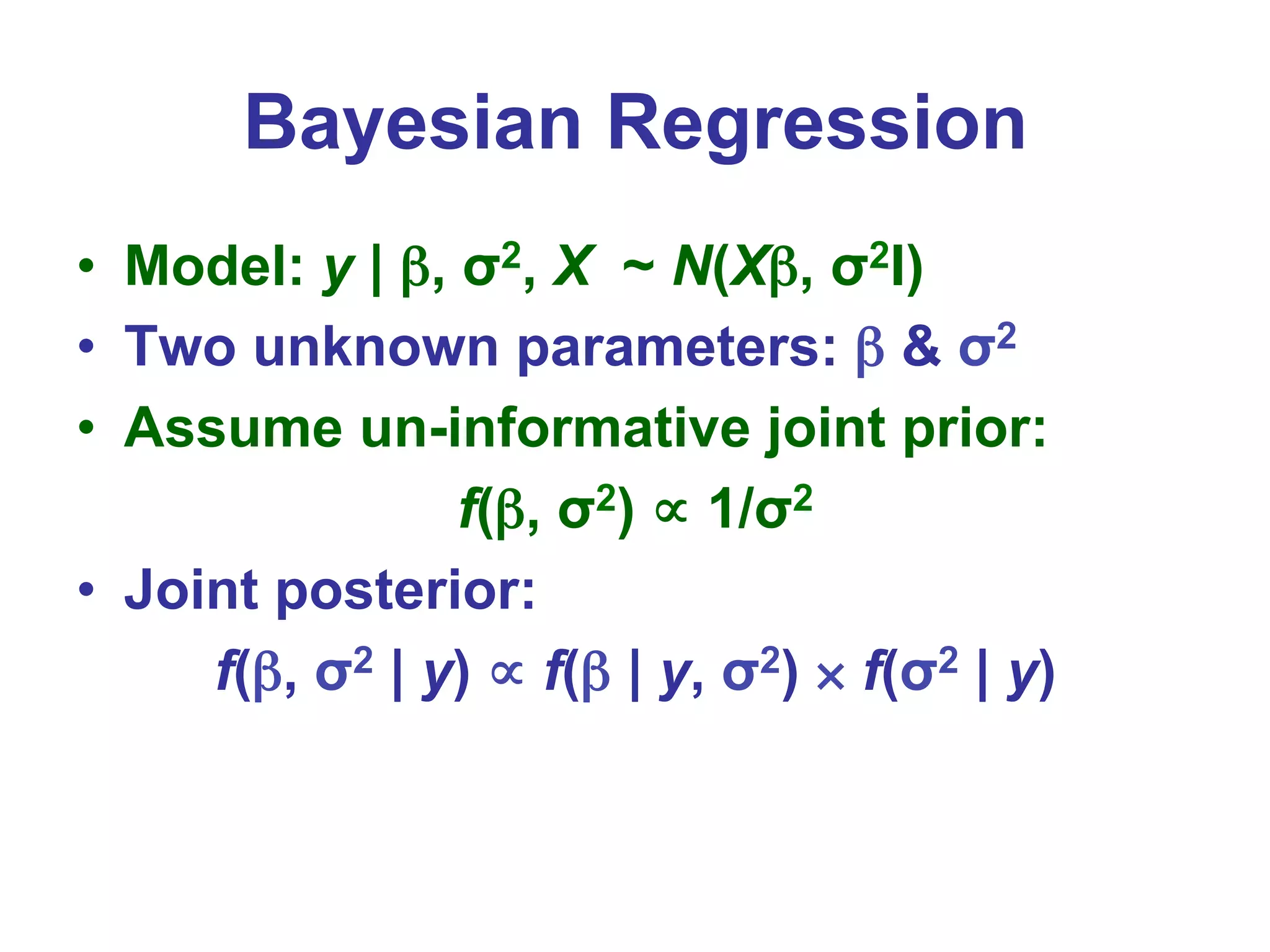
![Bayesian Regression
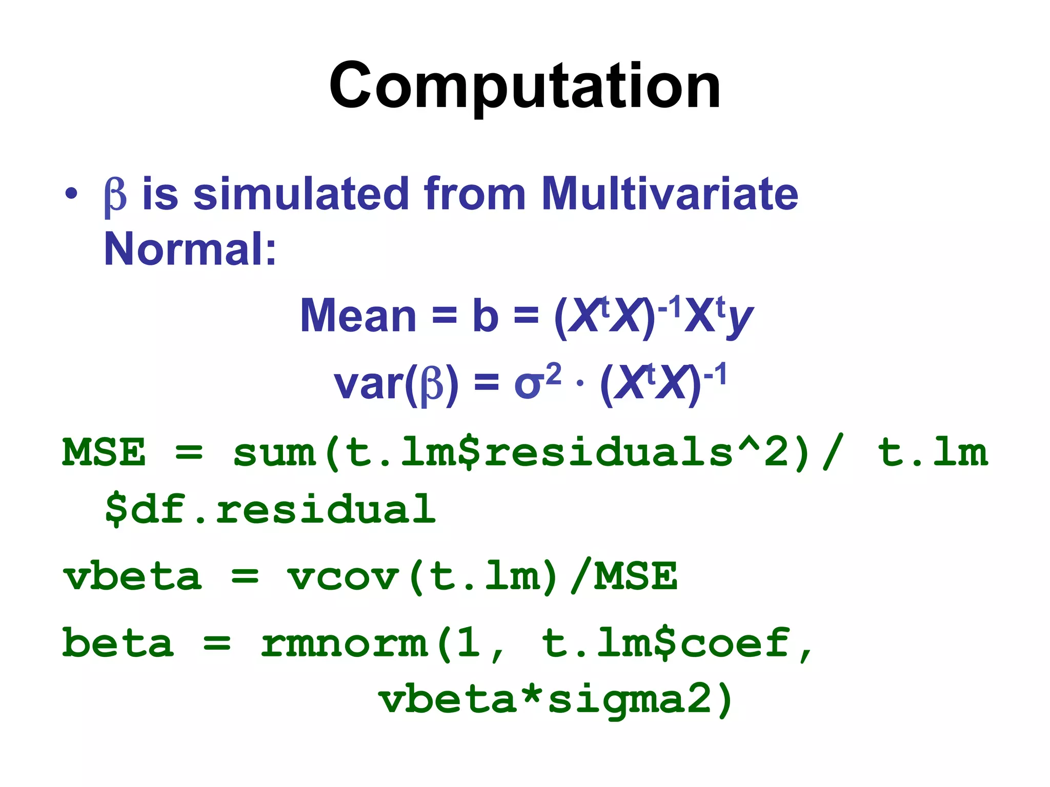
• Marginal posterior distribution of β,
conditional on error variance σ2 is
Multivariate Normal with:
Mean = b = (XtX)-1Xty
var(β) = σ2 ⋅ (XtX)-1
• Marginal posterior distribution of σ2 is
Inverse Gamma[(n - k)/2, S/2]
S = (y - Xb)t (y - Xb)](https://image.slidesharecdn.com/bayesianregressionintrowithr-130831160912-phpapp02/75/Bayesian-regression-intro-with-r-9-2048.jpg)
![Graphical Display
op = par(mfrow = c(2,2))
hist(par.sample$beta[, 2],
main= "Nesting",
xlab=expression(beta[1]))
hist(par.sample$beta[, 3],
main= "Size",
xlab=expression(beta[2]))](https://image.slidesharecdn.com/bayesianregressionintrowithr-130831160912-phpapp02/75/Bayesian-regression-intro-with-r-14-2048.jpg)
![Graphical Display
hist(par.sample$beta[, 4],
main= "Status",
xlab = expression(beta[3]))
hist(par.sample$sigma,
main= "Error SD",
xlab=expression(sigma))
par(op)](https://image.slidesharecdn.com/bayesianregressionintrowithr-130831160912-phpapp02/75/Bayesian-regression-intro-with-r-15-2048.jpg)
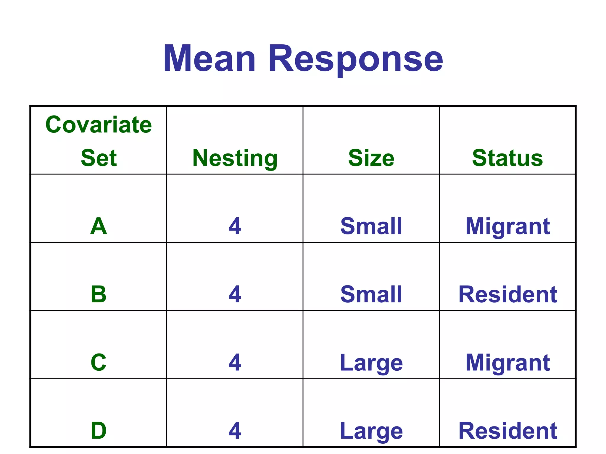
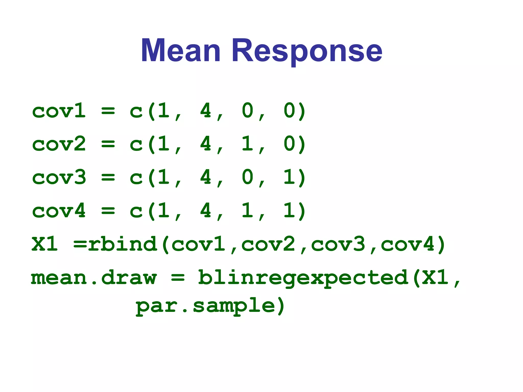
![Mean Response
op = par(mfrow = c(2,2))
hist(mean.draw[, 1],
main = "Covariate Set A",
xlab = "Log Time")
hist(mean.draw[, 2],
main = "Covariate Set B",
xlab = "Log Time")](https://image.slidesharecdn.com/bayesianregressionintrowithr-130831160912-phpapp02/75/Bayesian-regression-intro-with-r-19-2048.jpg)
![Mean Response
hist(mean.draw[, 3],
main = "Covariate Set C",
xlab = "Log Time")
hist(mean.draw[, 4],
main="Covariate Set D",
xlab="Log Time")
par(op)](https://image.slidesharecdn.com/bayesianregressionintrowithr-130831160912-phpapp02/75/Bayesian-regression-intro-with-r-20-2048.jpg)
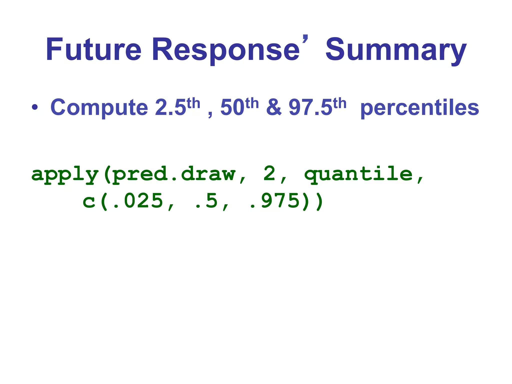
![Future Response
pred.draw=blinregpred(X1, par.sample)
op = par(mfrow = c(2,2))
hist(pred.draw[, 1], main="Covariate
Set A", xlab="Log Time")
hist(pred.draw[, 2], main="Covariate
Set B", xlab="Log Time")](https://image.slidesharecdn.com/bayesianregressionintrowithr-130831160912-phpapp02/75/Bayesian-regression-intro-with-r-22-2048.jpg)
![Future Response
hist(pred.draw[, 3],
main="Covariate Set C",
xlab="Log Time")
hist(pred.draw[, 2],
main="Covariate Set D",
xlab="Log Time")
par(op)](https://image.slidesharecdn.com/bayesianregressionintrowithr-130831160912-phpapp02/75/Bayesian-regression-intro-with-r-23-2048.jpg)

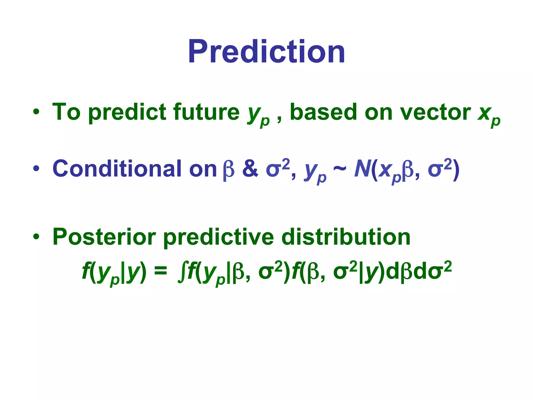
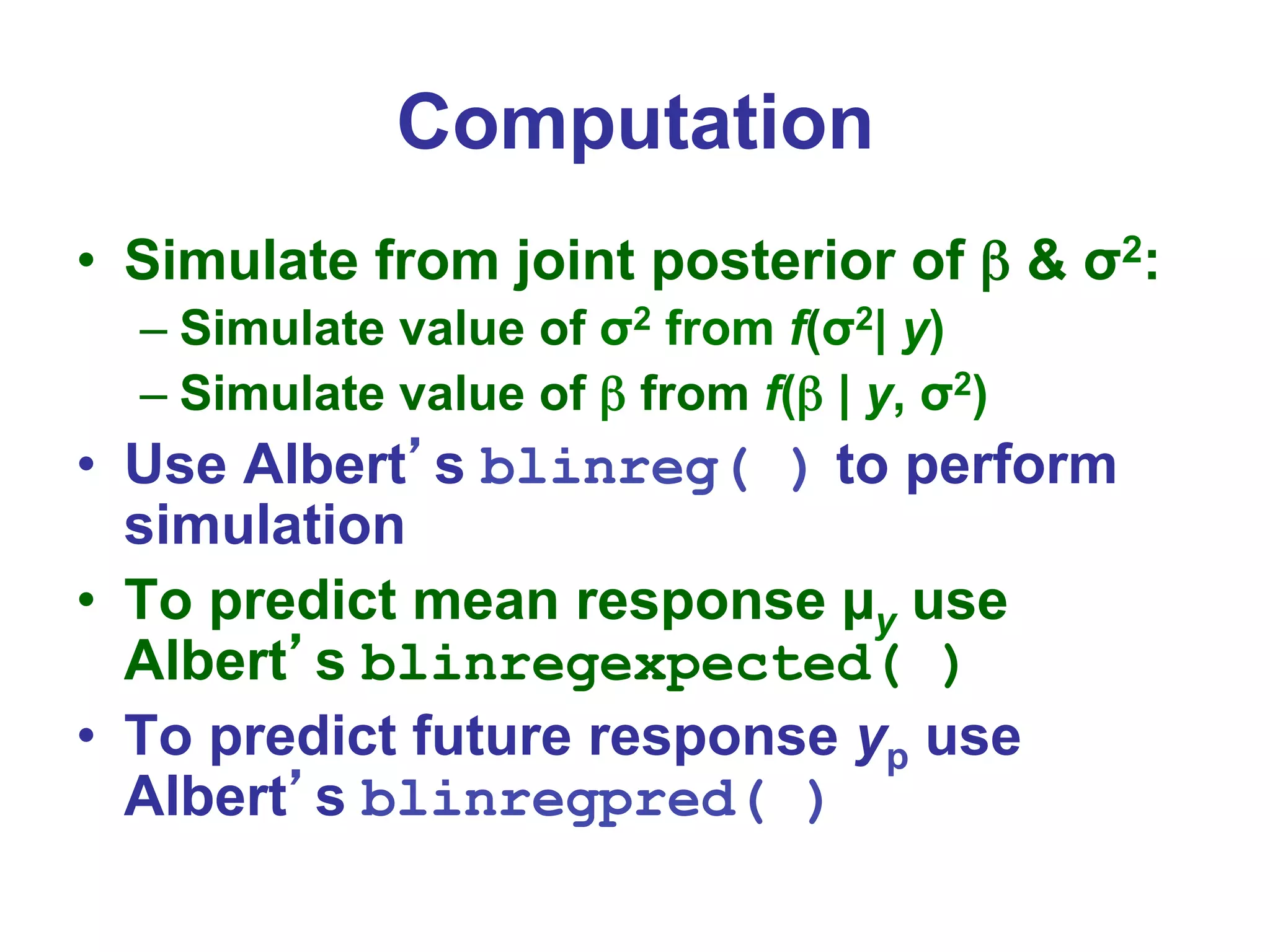
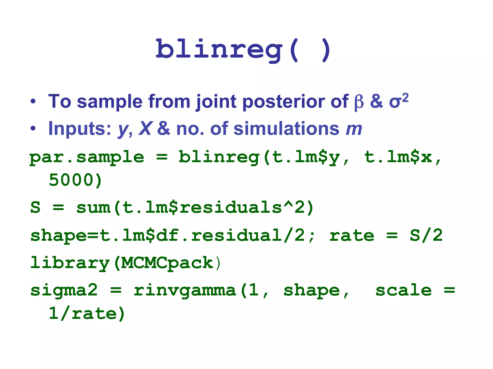
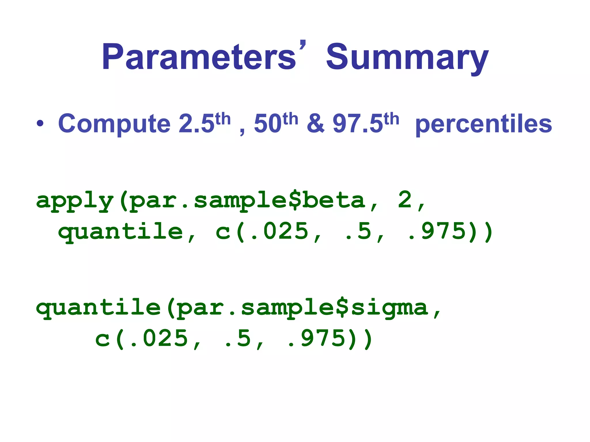
This document provides an introduction to Bayesian regression. It describes using a Bayesian approach to analyze a dataset on bird extinction times using multiple linear regression. Key steps include specifying prior distributions, computing the joint posterior distribution of the regression coefficients and error variance, and using MCMC methods like the blinreg() function to simulate values from the posterior. Graphical results show the distributions of coefficients and model predictions for different covariate patterns.


![[PRML 3.1~3.2] Linear Regression / Bias-Variance Decomposition](https://cdn.slidesharecdn.com/ss_thumbnails/bayesianlinearregressionpart1-170117134816-thumbnail.jpg?width=640&height=640&fit=bounds)