Problem Density Functions Generalized Density Functions The Bayesian Solution Summary
Universal Bayesian Measures
Joe Suzuki
Osaka University
IEEE International Symposium on Information Theory
Istanbul, Turky
July 8, 2013
1 / 19
Universal Bayesian Measures
Problem Density Functions Generalized Density Functions The Bayesian Solution Summary
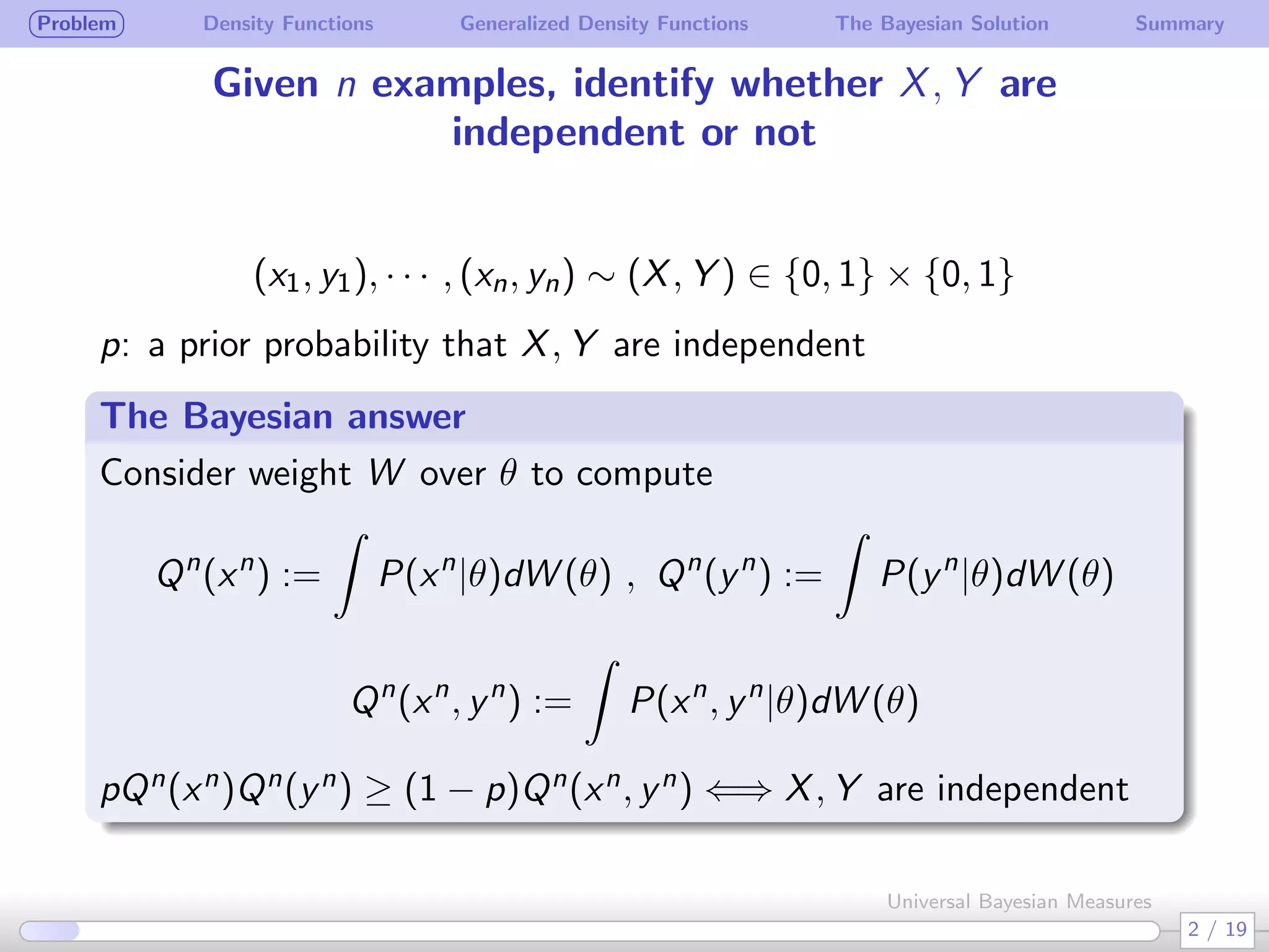
Given n examples, identify whether X, Y are
independent or not
(x1, y1), · · · , (xn, yn) ∼ (X, Y ) ∈ {0, 1} × {0, 1}
p: a prior probability that X, Y are independent
The Bayesian answer
Consider weight W over θ to compute
Qn
(xn
) :=
∫
P(xn
|θ)dW (θ) , Qn
(yn
) :=
∫
P(yn
|θ)dW (θ)
Qn
(xn
, yn
) :=
∫
P(xn
, yn
|θ)dW (θ)
pQn(xn)Qn(yn) ≥ (1 − p)Qn(xn, yn) ⇐⇒ X, Y are independent
2 / 19
Universal Bayesian Measures
Problem Density Functions Generalized Density Functions The Bayesian Solution Summary
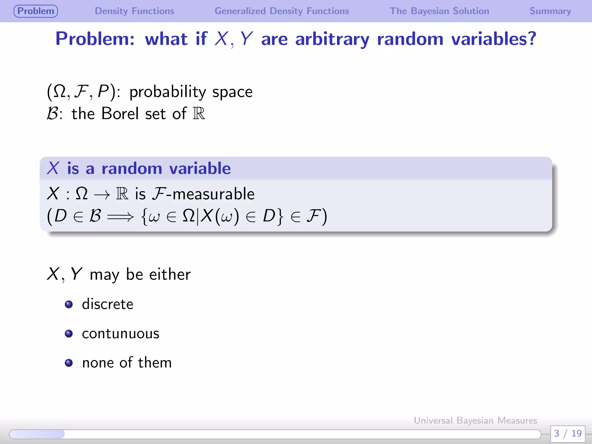
Problem: what if X, Y are arbitrary random variables?
(Ω, F, P): probability space
B: the Borel set of R
 
X is a random variable
.
.
X : Ω → R is F-measurable
(D ∈ B =⇒ {ω ∈ Ω|X(ω) ∈ D} ∈ F)
 
X, Y may be either
discrete
contunuous
none of them
3 / 19
Universal Bayesian Measures
Problem Density Functions Generalized Density Functions The Bayesian Solution Summary
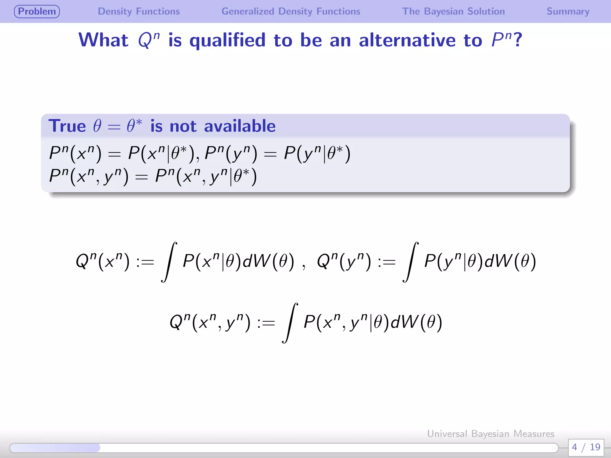
What Qn
is qualified to be an alternative to Pn
?
True θ = θ∗ is not available
.
.
Pn(xn) = P(xn|θ∗), Pn(yn) = P(yn|θ∗)
Pn(xn, yn) = Pn(xn, yn|θ∗)
Qn
(xn
) :=
∫
P(xn
|θ)dW (θ) , Qn
(yn
) :=
∫
P(yn
|θ)dW (θ)
Qn
(xn
, yn
) :=
∫
P(xn
, yn
|θ)dW (θ)
4 / 19
Universal Bayesian Measures
Problem Density Functions Generalized Density Functions The Bayesian Solution Summary
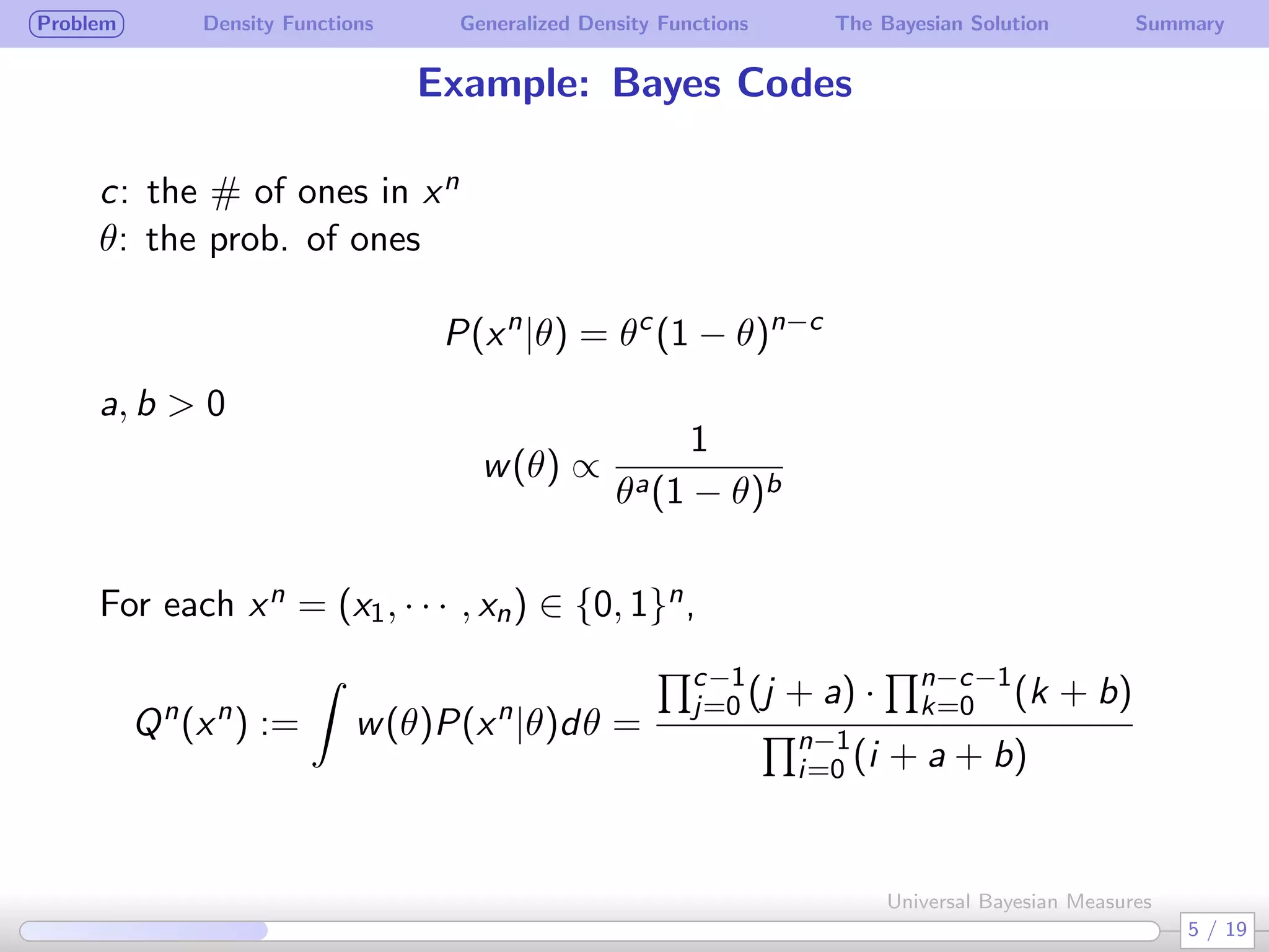
Example: Bayes Codes
c: the # of ones in xn
θ: the prob. of ones
P(xn
|θ) = θc
(1 − θ)n−c
a, b > 0
w(θ) ∝
1
θa(1 − θ)b
 
For each xn = (x1, · · · , xn) ∈ {0, 1}n,
Qn
(xn
) :=
∫
w(θ)P(xn
|θ)dθ =
∏c−1
j=0 (j + a) ·
∏n−c−1
k=0 (k + b)
∏n−1
i=0 (i + a + b)
5 / 19
Universal Bayesian Measures
Problem Density Functions Generalized Density Functions The Bayesian Solution Summary
Universal Coding/Measures
If we choose
a = b = 1/2
(Krichevsky-Trofimov) and xn is i.i.d. emitted by
Pn
(xn
|θ) =
n∏
i=1
P(xi ) , P(xi ) = θ, 1 − θ
then, for any P, almost surely,
−
1
n
log Qn
(xn
) → H :=
∑
x∈A
−P(x) log P(x)
From Shannon McMillian Breiman, for any P,
−
1
n
log Pn
(xn
|θ) =
1
n
n∑
i=1
− log P(xi ) → E[− log P(xi )] = H
6 / 19
Universal Bayesian Measures
Problem Density Functions Generalized Density Functions The Bayesian Solution Summary
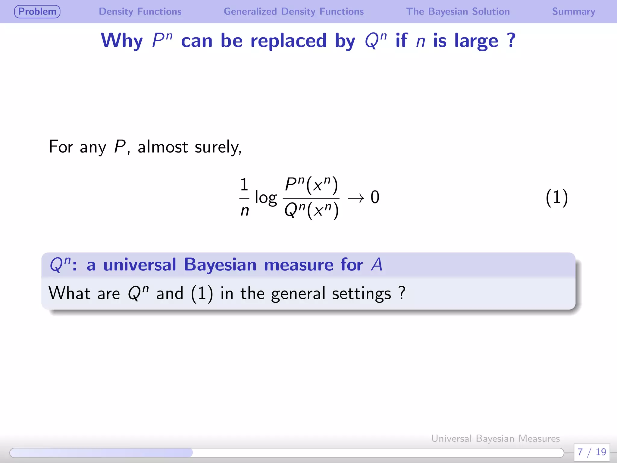
Why Pn
can be replaced by Qn
if n is large ?
For any P, almost surely,
1
n
log
Pn(xn)
Qn(xn)
→ 0 (1)
Qn: a universal Bayesian measure for A
.
What are Qn and (1) in the general settings ?
7 / 19
Universal Bayesian Measures
Problem Density Functions Generalized Density Functions The Bayesian Solution Summary
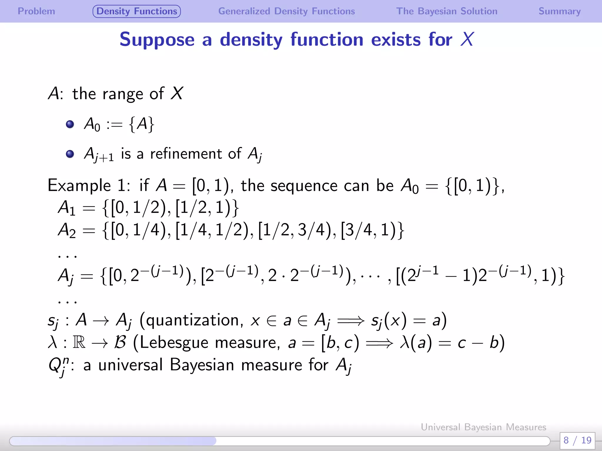
Suppose a density function exists for X
A: the range of X
A0 := {A}
Aj+1 is a refinement of Aj
Example 1: if A = [0, 1), the sequence can be A0 = {[0, 1)},
A1 = {[0, 1/2), [1/2, 1)}
A2 = {[0, 1/4), [1/4, 1/2), [1/2, 3/4), [3/4, 1)}
. . .
Aj = {[0, 2−(j−1)), [2−(j−1), 2 · 2−(j−1)), · · · , [(2j−1 − 1)2−(j−1), 1)}
. . .
sj : A → Aj (quantization, x ∈ a ∈ Aj =⇒ sj (x) = a)
λ : R → B (Lebesgue measure, a = [b, c) =⇒ λ(a) = c − b)
Qn
j : a universal Bayesian measure for Aj
8 / 19
Universal Bayesian Measures
Problem Density Functions Generalized Density Functions The Bayesian Solution Summary
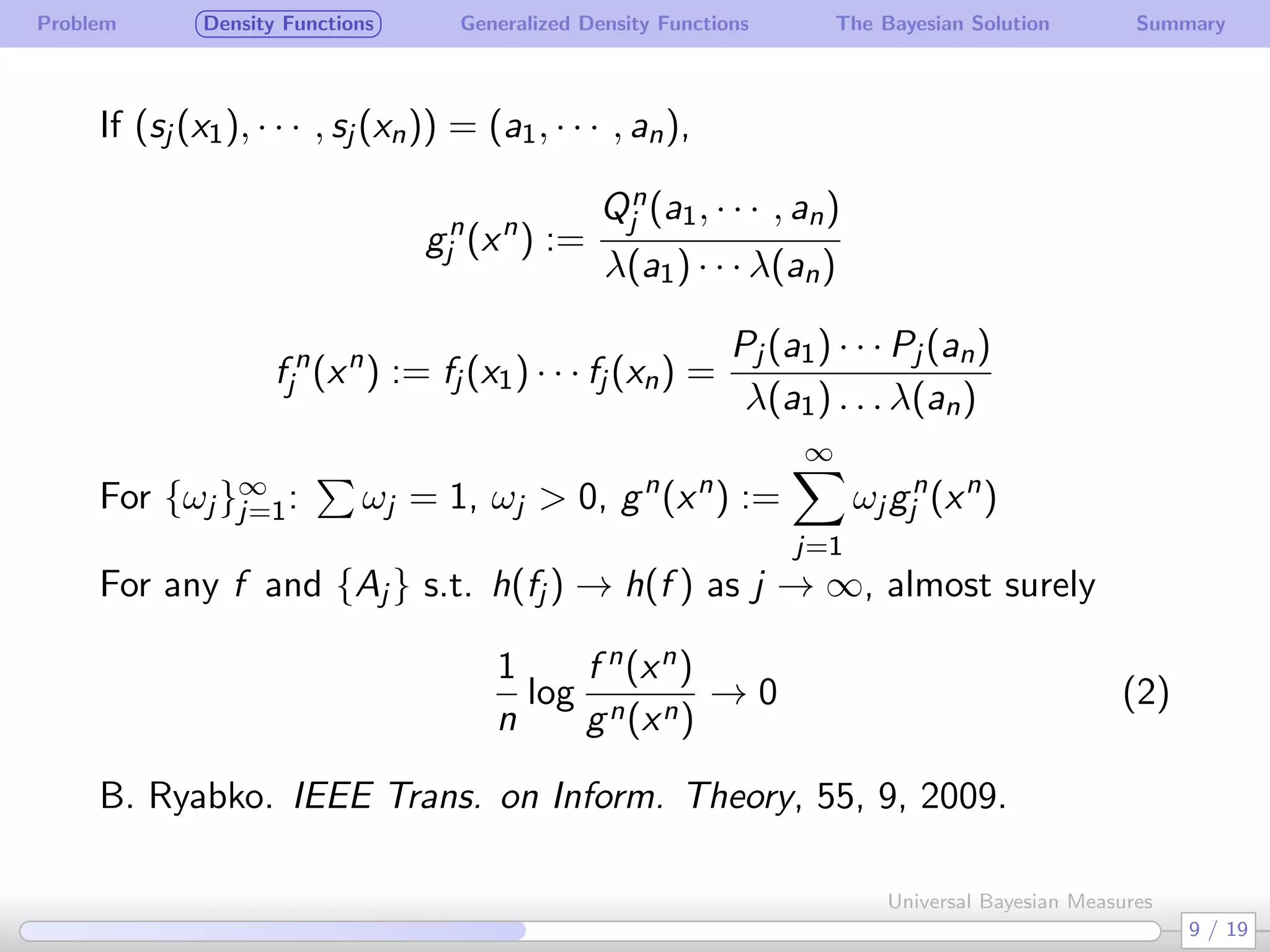
If (sj (x1), · · · , sj (xn)) = (a1, · · · , an),
gn
j (xn
) :=
Qn
j (a1, · · · , an)
λ(a1) · · · λ(an)
f n
j (xn
) := fj (x1) · · · fj (xn) =
Pj (a1) · · · Pj (an)
λ(a1) . . . λ(an)
For {ωj }∞
j=1:
∑
ωj = 1, ωj > 0, gn
(xn
) :=
∞∑
j=1
ωj gn
j (xn
)
For any f and {Aj } s.t. h(fj ) → h(f ) as j → ∞, almost surely
1
n
log
f n(xn)
gn(xn)
→ 0 (2)
B. Ryabko. IEEE Trans. on Inform. Theory, 55, 9, 2009.
9 / 19
Universal Bayesian Measures
Problem Density Functions Generalized Density Functions The Bayesian Solution Summary
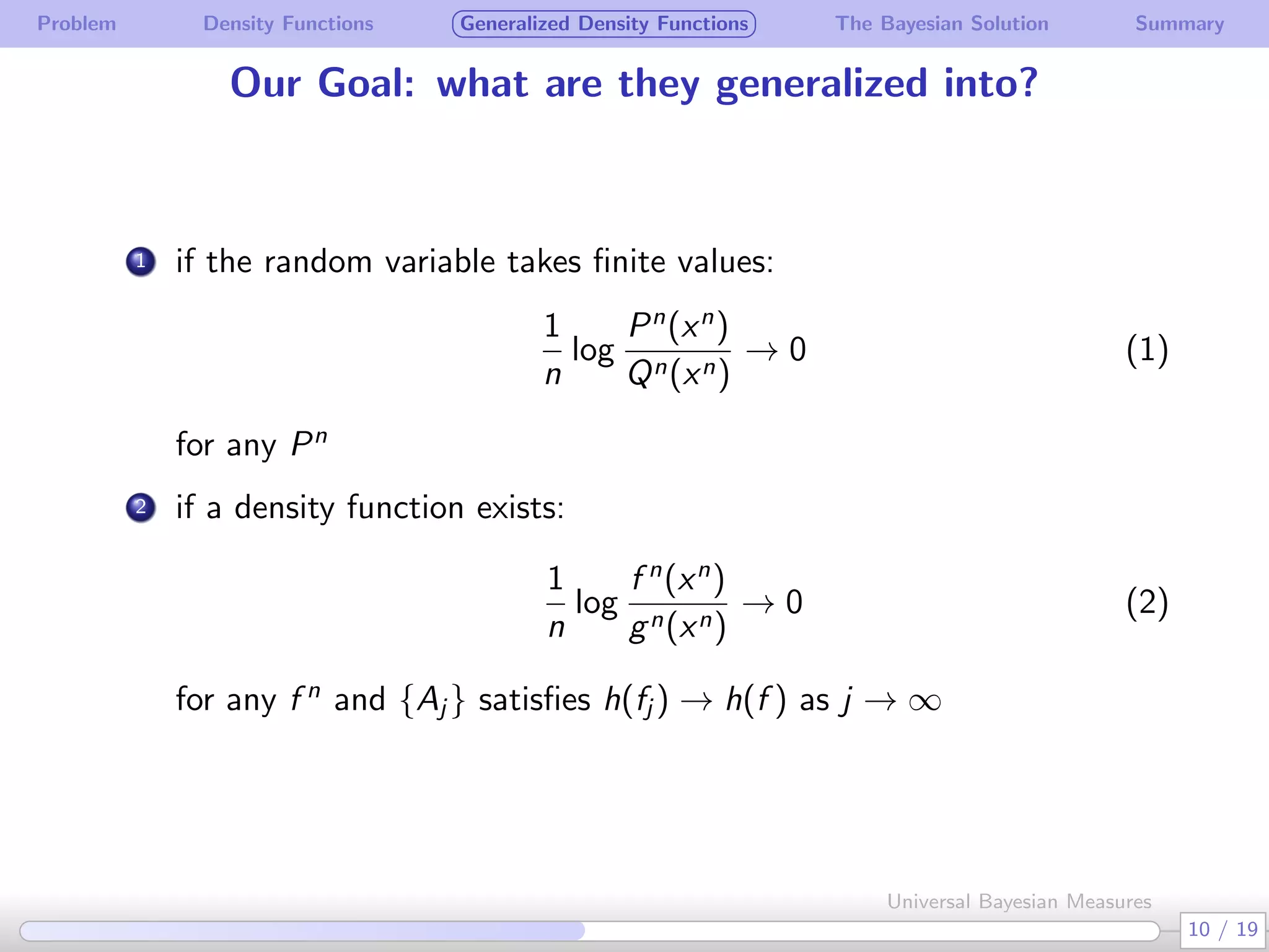
Our Goal: what are they generalized into?
. 1 if the random variable takes finite values:
1
n
log
Pn
(xn
)
Qn(xn)
→ 0 (1)
for any Pn
.
2 if a density function exists:
1
n
log
f n
(xn
)
gn(xn)
→ 0 (2)
for any f n
and {Aj } satisfies h(fj ) → h(f ) as j → ∞
10 / 19
Universal Bayesian Measures
Problem Density Functions Generalized Density Functions The Bayesian Solution Summary
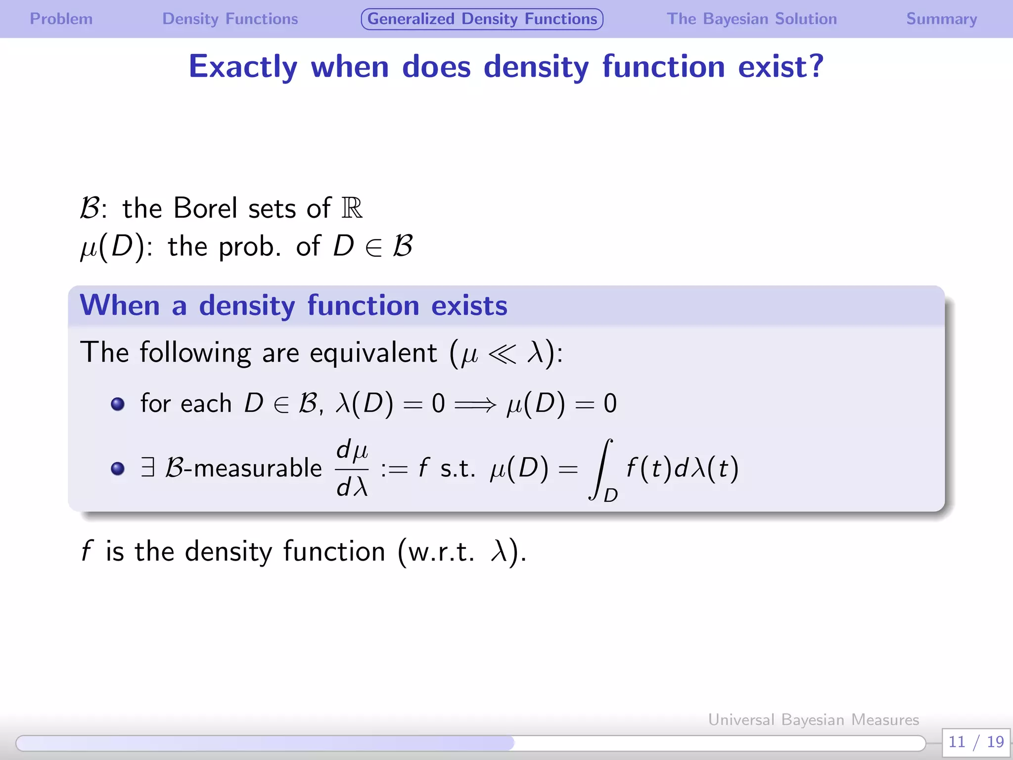
Exactly when does density function exist?
B: the Borel sets of R
µ(D): the prob. of D ∈ B
When a density function exists
.
The following are equivalent (µ ≪ λ):
for each D ∈ B, λ(D) = 0 =⇒ µ(D) = 0
∃ B-measurable
dµ
dλ
:= f s.t. µ(D) =
∫
D
f (t)dλ(t)
f is the density function (w.r.t. λ).
11 / 19
Universal Bayesian Measures
Problem Density Functions Generalized Density Functions The Bayesian Solution Summary
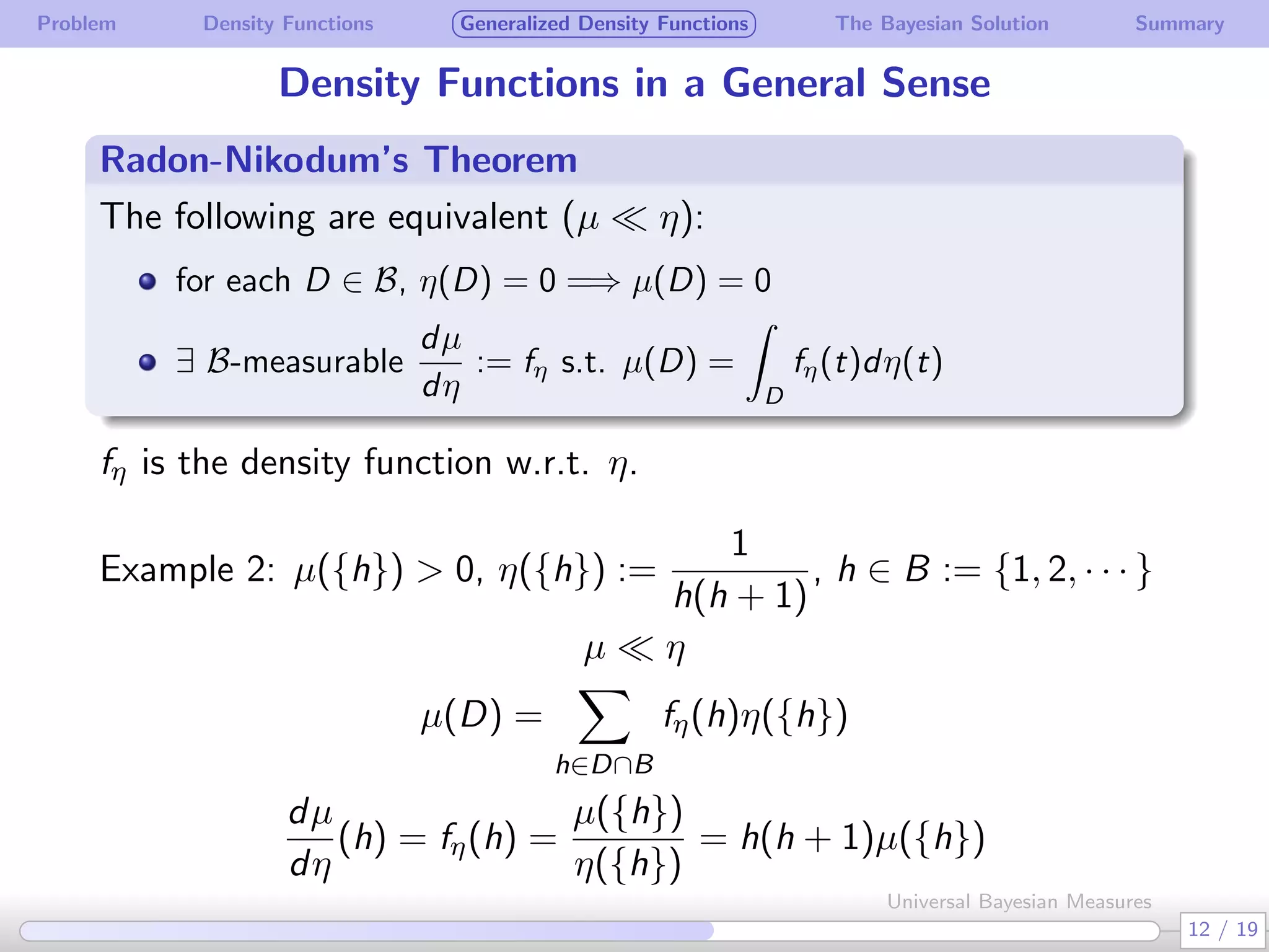
Density Functions in a General Sense
Radon-Nikodum’s Theorem
.
.
The following are equivalent (µ ≪ η):
for each D ∈ B, η(D) = 0 =⇒ µ(D) = 0
∃ B-measurable
dµ
dη
:= fη s.t. µ(D) =
∫
D
fη(t)dη(t)
fη is the density function w.r.t. η.
 
Example 2: µ({h}) > 0, η({h}) :=
1
h(h + 1)
, h ∈ B := {1, 2, · · · }
µ ≪ η
µ(D) =
∑
h∈D∩B
fη(h)η({h})
dµ
dη
(h) = fη(h) =
µ({h})
η({h})
= h(h + 1)µ({h})
12 / 19
Universal Bayesian Measures
Problem Density Functions Generalized Density Functions The Bayesian Solution Summary
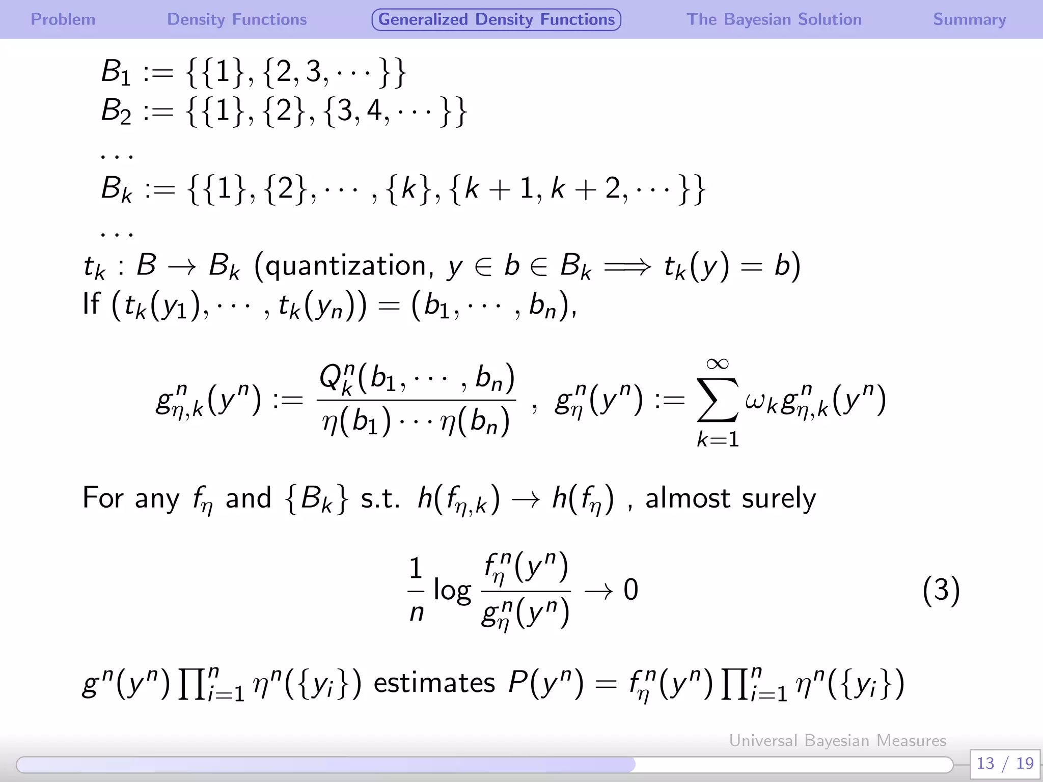
B1 := {{1}, {2, 3, · · · }}
B2 := {{1}, {2}, {3, 4, · · · }}
. . .
Bk := {{1}, {2}, · · · , {k}, {k + 1, k + 2, · · · }}
. . .
tk : B → Bk (quantization, y ∈ b ∈ Bk =⇒ tk(y) = b)
If (tk(y1), · · · , tk(yn)) = (b1, · · · , bn),
gn
η,k(yn
) :=
Qn
k (b1, · · · , bn)
η(b1) · · · η(bn)
, gn
η (yn
) :=
∞∑
k=1
ωkgn
η,k(yn
)
For any fη and {Bk} s.t. h(fη,k) → h(fη) , almost surely
1
n
log
f n
η (yn)
gn
η (yn)
→ 0 (3)
gn(yn)
∏n
i=1 ηn({yi }) estimates P(yn) = f n
η (yn)
∏n
i=1 ηn({yi })
13 / 19
Universal Bayesian Measures
Problem Density Functions Generalized Density Functions The Bayesian Solution Summary
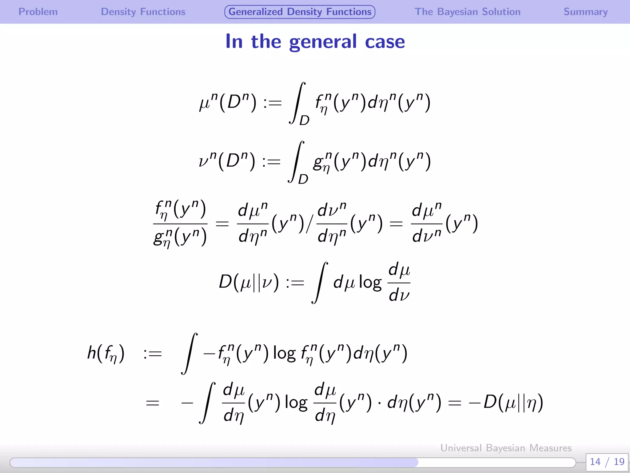
In the general case
µn
(Dn
) :=
∫
D
f n
η (yn
)dηn
(yn
)
νn
(Dn
) :=
∫
D
gn
η (yn
)dηn
(yn
)
f n
η (yn)
gn
η (yn)
=
dµn
dηn
(yn
)/
dνn
dηn
(yn
) =
dµn
dνn
(yn
)
D(µ||ν) :=
∫
dµ log
dµ
dν
h(fη) :=
∫
−f n
η (yn
) log f n
η (yn
)dη(yn
)
= −
∫
dµ
dη
(yn
) log
dµ
dη
(yn
) · dη(yn
) = −D(µ||η)
14 / 19
Universal Bayesian Measures
Problem Density Functions Generalized Density Functions The Bayesian Solution Summary
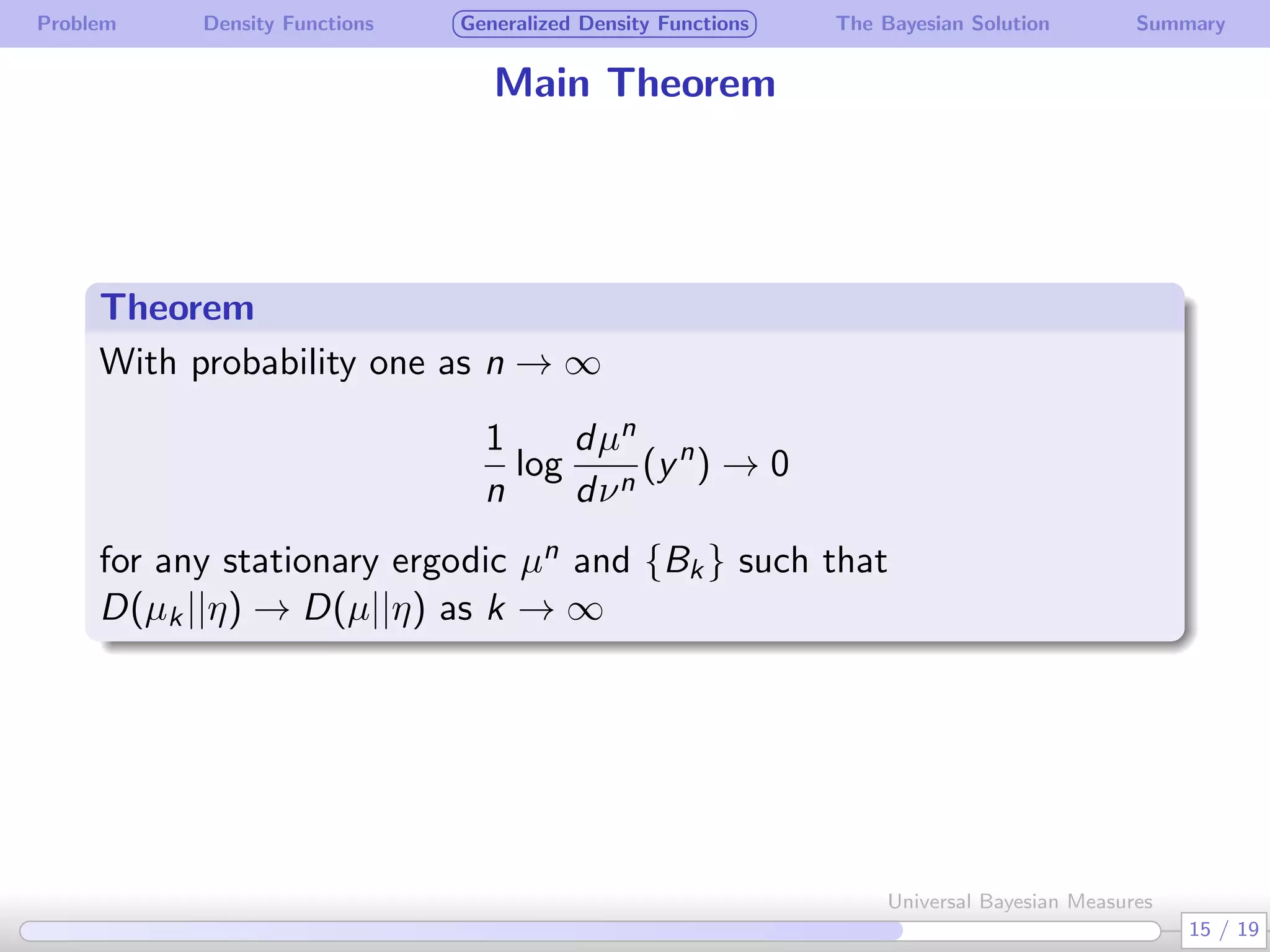
Main Theorem
Theorem
.
With probability one as n → ∞
1
n
log
dµn
dνn
(yn
) → 0
for any stationary ergodic µn and {Bk} such that
D(µk||η) → D(µ||η) as k → ∞
15 / 19
Universal Bayesian Measures
Problem Density Functions Generalized Density Functions The Bayesian Solution Summary
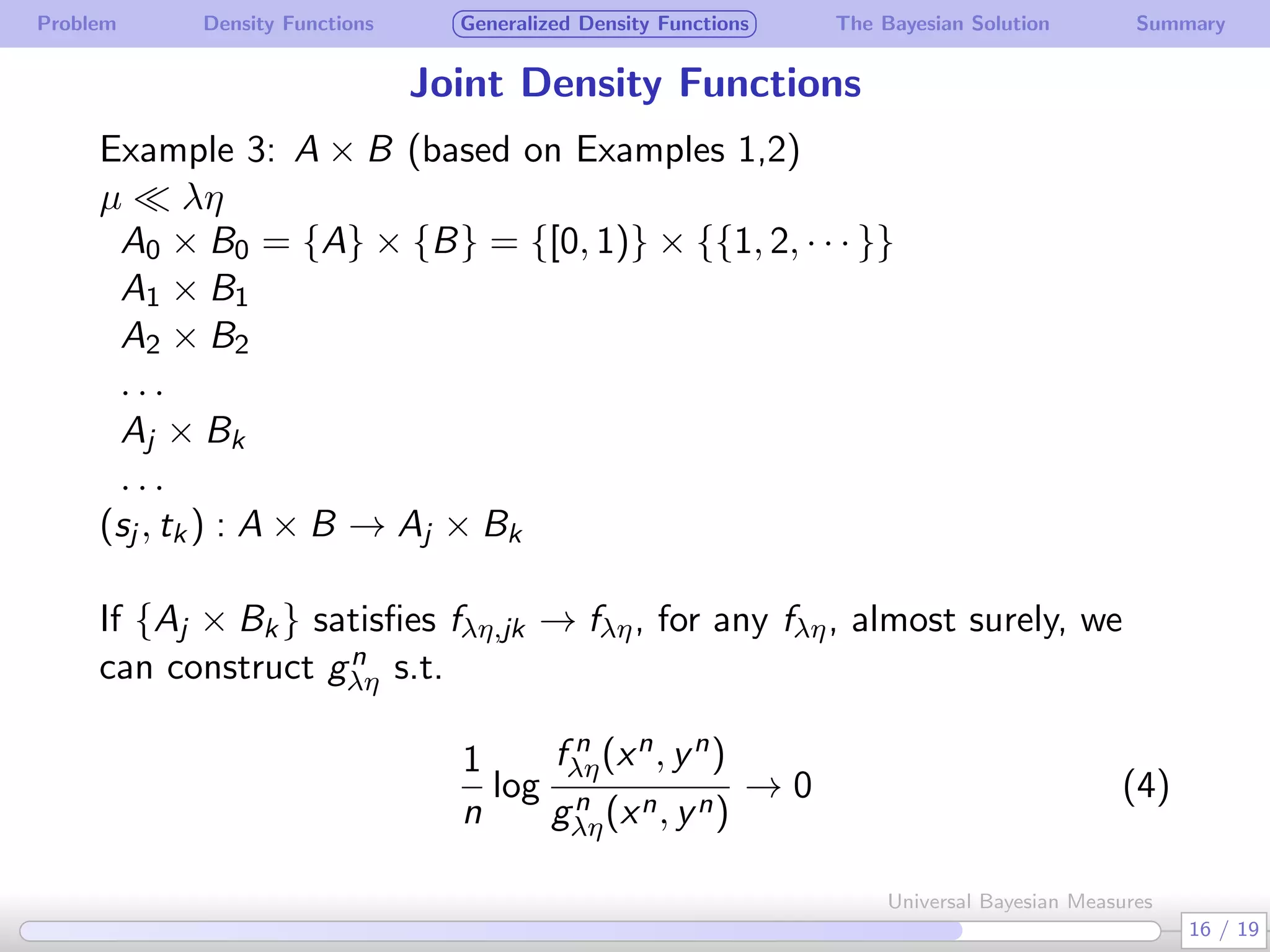
Joint Density Functions
Example 3: A × B (based on Examples 1,2)
µ ≪ λη
A0 × B0 = {A} × {B} = {[0, 1)} × {{1, 2, · · · }}
A1 × B1
A2 × B2
. . .
Aj × Bk
. . .
(sj , tk) : A × B → Aj × Bk
 
If {Aj × Bk} satisfies fλη,jk → fλη, for any fλη, almost surely, we
can construct gn
λη s.t.
1
n
log
f n
λη(xn, yn)
gn
λη(xn, yn)
→ 0 (4)
16 / 19
Universal Bayesian Measures
Problem Density Functions Generalized Density Functions The Bayesian Solution Summary
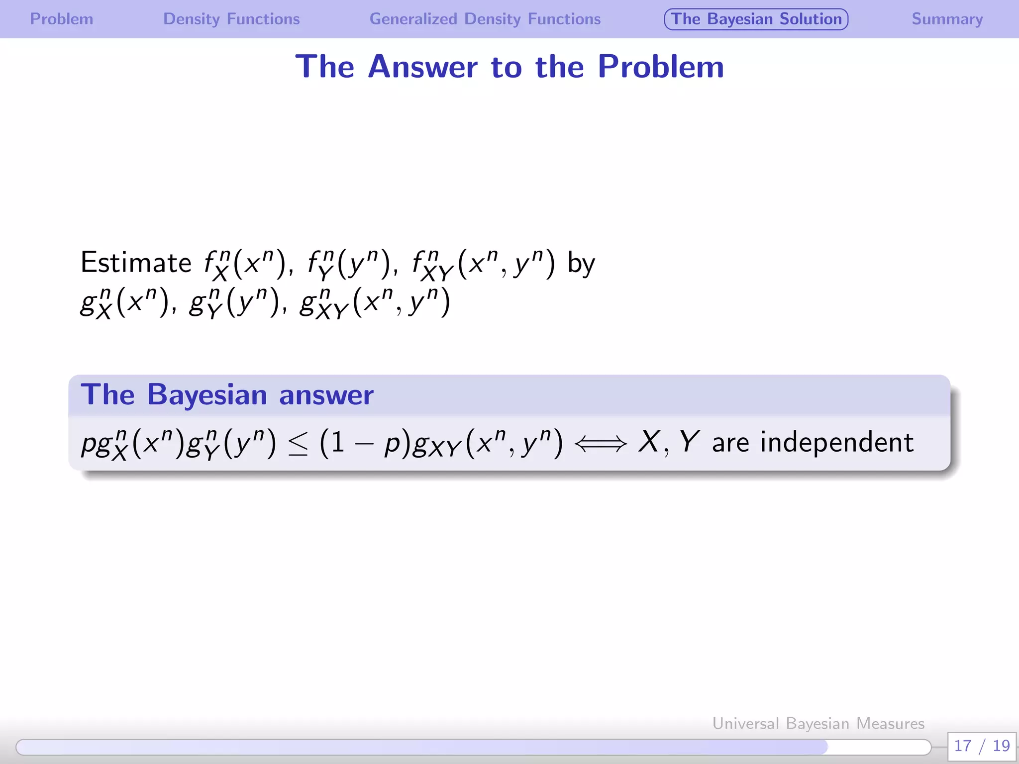
The Answer to the Problem
Estimate f n
X (xn), f n
Y (yn), f n
XY (xn, yn) by
gn
X (xn), gn
Y (yn), gn
XY (xn, yn)
 
The Bayesian answer
.
.
pgn
X (xn)gn
Y (yn) ≤ (1 − p)gXY (xn, yn) ⇐⇒ X, Y are independent
17 / 19
Universal Bayesian Measures
Problem Density Functions Generalized Density Functions The Bayesian Solution Summary
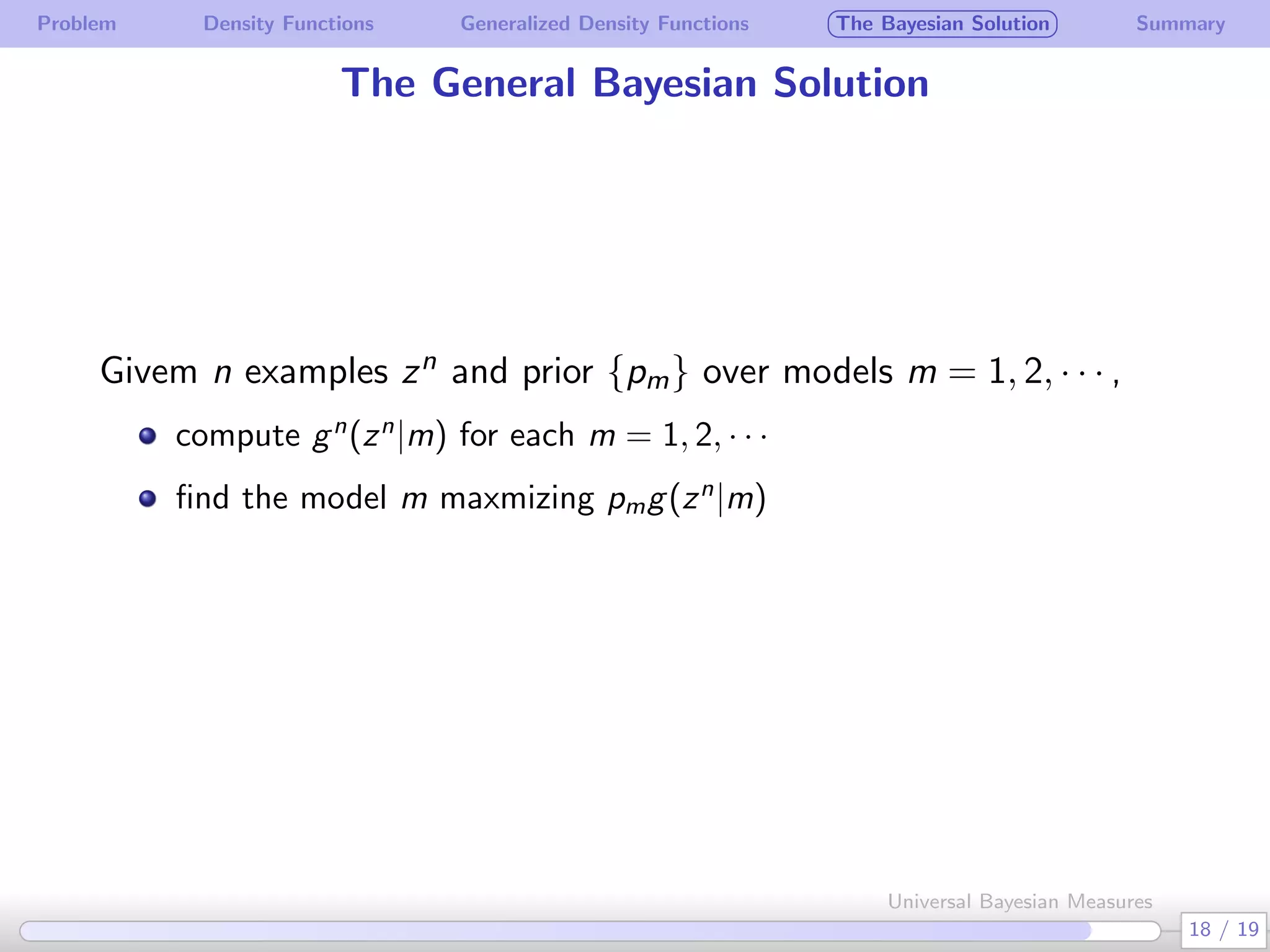
The General Bayesian Solution
Givem n examples zn and prior {pm} over models m = 1, 2, · · · ,
compute gn
(zn
|m) for each m = 1, 2, · · ·
find the model m maxmizing pmg(zn
|m)
18 / 19
Universal Bayesian Measures
Problem Density Functions Generalized Density Functions The Bayesian Solution Summary
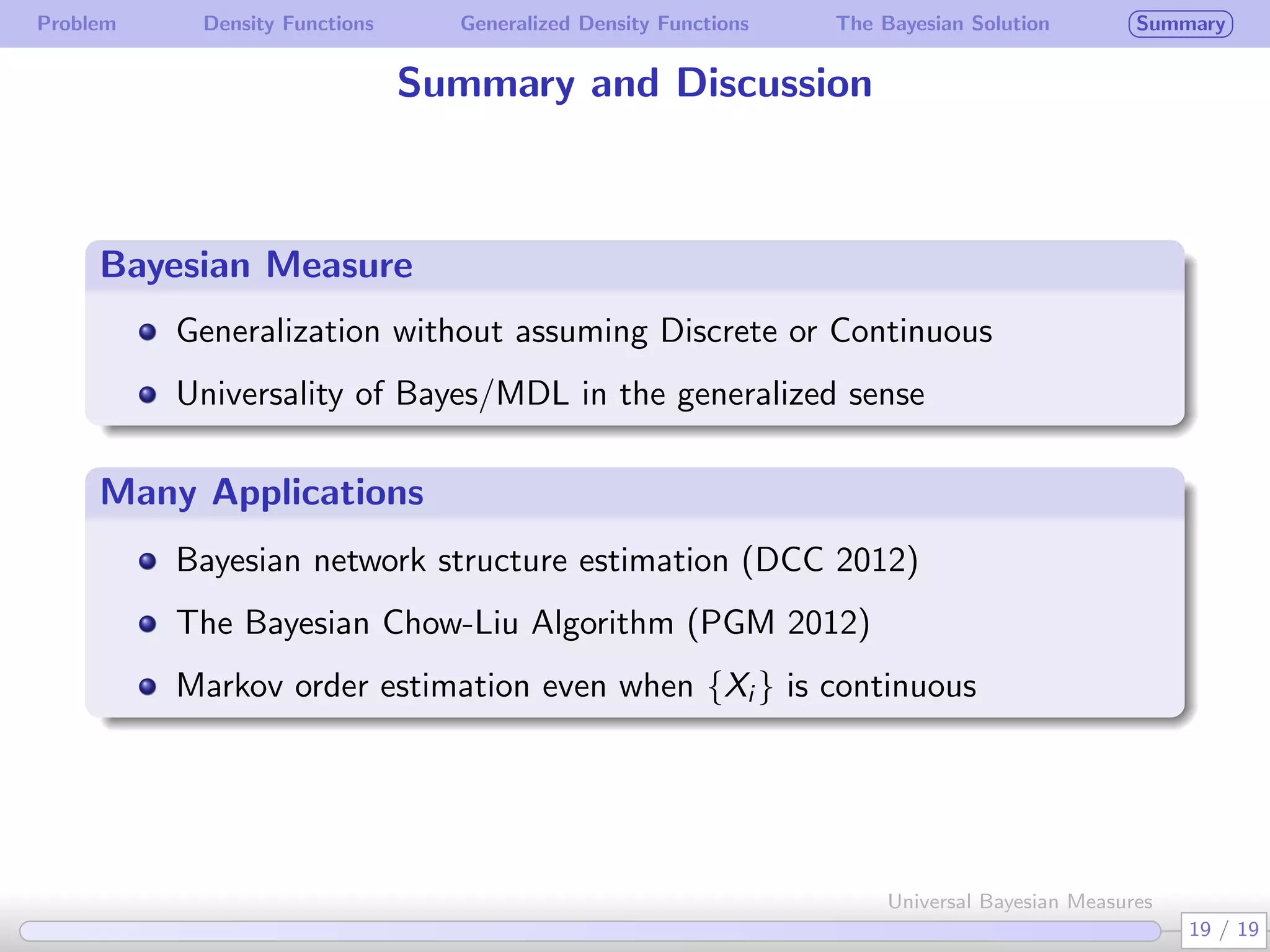
Summary and Discussion
Bayesian Measure
.
.
Generalization without assuming Discrete or Continuous
Universality of Bayes/MDL in the generalized sense
Many Applications
Bayesian network structure estimation (DCC 2012)
The Bayesian Chow-Liu Algorithm (PGM 2012)
Markov order estimation even when {Xi } is continuous
19 / 19
Universal Bayesian Measures

2013 IEEE International Symposium on Information Theory

  • 1.
    Problem Density FunctionsGeneralized Density Functions The Bayesian Solution Summary Universal Bayesian Measures Joe Suzuki Osaka University IEEE International Symposium on Information Theory Istanbul, Turky July 8, 2013 1 / 19 Universal Bayesian Measures
  • 2.
    Problem Density FunctionsGeneralized Density Functions The Bayesian Solution Summary Given n examples, identify whether X, Y are independent or not (x1, y1), · · · , (xn, yn) ∼ (X, Y ) ∈ {0, 1} × {0, 1} p: a prior probability that X, Y are independent The Bayesian answer Consider weight W over θ to compute Qn (xn ) := ∫ P(xn |θ)dW (θ) , Qn (yn ) := ∫ P(yn |θ)dW (θ) Qn (xn , yn ) := ∫ P(xn , yn |θ)dW (θ) pQn(xn)Qn(yn) ≥ (1 − p)Qn(xn, yn) ⇐⇒ X, Y are independent 2 / 19 Universal Bayesian Measures
  • 3.
    Problem Density FunctionsGeneralized Density Functions The Bayesian Solution Summary Problem: what if X, Y are arbitrary random variables? (Ω, F, P): probability space B: the Borel set of R   X is a random variable . . X : Ω → R is F-measurable (D ∈ B =⇒ {ω ∈ Ω|X(ω) ∈ D} ∈ F)   X, Y may be either discrete contunuous none of them 3 / 19 Universal Bayesian Measures
  • 4.
    Problem Density FunctionsGeneralized Density Functions The Bayesian Solution Summary What Qn is qualified to be an alternative to Pn ? True θ = θ∗ is not available . . Pn(xn) = P(xn|θ∗), Pn(yn) = P(yn|θ∗) Pn(xn, yn) = Pn(xn, yn|θ∗) Qn (xn ) := ∫ P(xn |θ)dW (θ) , Qn (yn ) := ∫ P(yn |θ)dW (θ) Qn (xn , yn ) := ∫ P(xn , yn |θ)dW (θ) 4 / 19 Universal Bayesian Measures
  • 5.
    Problem Density FunctionsGeneralized Density Functions The Bayesian Solution Summary Example: Bayes Codes c: the # of ones in xn θ: the prob. of ones P(xn |θ) = θc (1 − θ)n−c a, b > 0 w(θ) ∝ 1 θa(1 − θ)b   For each xn = (x1, · · · , xn) ∈ {0, 1}n, Qn (xn ) := ∫ w(θ)P(xn |θ)dθ = ∏c−1 j=0 (j + a) · ∏n−c−1 k=0 (k + b) ∏n−1 i=0 (i + a + b) 5 / 19 Universal Bayesian Measures
  • 6.
    Problem Density FunctionsGeneralized Density Functions The Bayesian Solution Summary Universal Coding/Measures If we choose a = b = 1/2 (Krichevsky-Trofimov) and xn is i.i.d. emitted by Pn (xn |θ) = n∏ i=1 P(xi ) , P(xi ) = θ, 1 − θ then, for any P, almost surely, − 1 n log Qn (xn ) → H := ∑ x∈A −P(x) log P(x) From Shannon McMillian Breiman, for any P, − 1 n log Pn (xn |θ) = 1 n n∑ i=1 − log P(xi ) → E[− log P(xi )] = H 6 / 19 Universal Bayesian Measures
  • 7.
    Problem Density FunctionsGeneralized Density Functions The Bayesian Solution Summary Why Pn can be replaced by Qn if n is large ? For any P, almost surely, 1 n log Pn(xn) Qn(xn) → 0 (1) Qn: a universal Bayesian measure for A . What are Qn and (1) in the general settings ? 7 / 19 Universal Bayesian Measures
  • 8.
    Problem Density FunctionsGeneralized Density Functions The Bayesian Solution Summary Suppose a density function exists for X A: the range of X A0 := {A} Aj+1 is a refinement of Aj Example 1: if A = [0, 1), the sequence can be A0 = {[0, 1)}, A1 = {[0, 1/2), [1/2, 1)} A2 = {[0, 1/4), [1/4, 1/2), [1/2, 3/4), [3/4, 1)} . . . Aj = {[0, 2−(j−1)), [2−(j−1), 2 · 2−(j−1)), · · · , [(2j−1 − 1)2−(j−1), 1)} . . . sj : A → Aj (quantization, x ∈ a ∈ Aj =⇒ sj (x) = a) λ : R → B (Lebesgue measure, a = [b, c) =⇒ λ(a) = c − b) Qn j : a universal Bayesian measure for Aj 8 / 19 Universal Bayesian Measures
  • 9.
    Problem Density FunctionsGeneralized Density Functions The Bayesian Solution Summary If (sj (x1), · · · , sj (xn)) = (a1, · · · , an), gn j (xn ) := Qn j (a1, · · · , an) λ(a1) · · · λ(an) f n j (xn ) := fj (x1) · · · fj (xn) = Pj (a1) · · · Pj (an) λ(a1) . . . λ(an) For {ωj }∞ j=1: ∑ ωj = 1, ωj > 0, gn (xn ) := ∞∑ j=1 ωj gn j (xn ) For any f and {Aj } s.t. h(fj ) → h(f ) as j → ∞, almost surely 1 n log f n(xn) gn(xn) → 0 (2) B. Ryabko. IEEE Trans. on Inform. Theory, 55, 9, 2009. 9 / 19 Universal Bayesian Measures
  • 10.
    Problem Density FunctionsGeneralized Density Functions The Bayesian Solution Summary Our Goal: what are they generalized into? . 1 if the random variable takes finite values: 1 n log Pn (xn ) Qn(xn) → 0 (1) for any Pn . 2 if a density function exists: 1 n log f n (xn ) gn(xn) → 0 (2) for any f n and {Aj } satisfies h(fj ) → h(f ) as j → ∞ 10 / 19 Universal Bayesian Measures
  • 11.
    Problem Density FunctionsGeneralized Density Functions The Bayesian Solution Summary Exactly when does density function exist? B: the Borel sets of R µ(D): the prob. of D ∈ B When a density function exists . The following are equivalent (µ ≪ λ): for each D ∈ B, λ(D) = 0 =⇒ µ(D) = 0 ∃ B-measurable dµ dλ := f s.t. µ(D) = ∫ D f (t)dλ(t) f is the density function (w.r.t. λ). 11 / 19 Universal Bayesian Measures
  • 12.
    Problem Density FunctionsGeneralized Density Functions The Bayesian Solution Summary Density Functions in a General Sense Radon-Nikodum’s Theorem . . The following are equivalent (µ ≪ η): for each D ∈ B, η(D) = 0 =⇒ µ(D) = 0 ∃ B-measurable dµ dη := fη s.t. µ(D) = ∫ D fη(t)dη(t) fη is the density function w.r.t. η.   Example 2: µ({h}) > 0, η({h}) := 1 h(h + 1) , h ∈ B := {1, 2, · · · } µ ≪ η µ(D) = ∑ h∈D∩B fη(h)η({h}) dµ dη (h) = fη(h) = µ({h}) η({h}) = h(h + 1)µ({h}) 12 / 19 Universal Bayesian Measures
  • 13.
    Problem Density FunctionsGeneralized Density Functions The Bayesian Solution Summary B1 := {{1}, {2, 3, · · · }} B2 := {{1}, {2}, {3, 4, · · · }} . . . Bk := {{1}, {2}, · · · , {k}, {k + 1, k + 2, · · · }} . . . tk : B → Bk (quantization, y ∈ b ∈ Bk =⇒ tk(y) = b) If (tk(y1), · · · , tk(yn)) = (b1, · · · , bn), gn η,k(yn ) := Qn k (b1, · · · , bn) η(b1) · · · η(bn) , gn η (yn ) := ∞∑ k=1 ωkgn η,k(yn ) For any fη and {Bk} s.t. h(fη,k) → h(fη) , almost surely 1 n log f n η (yn) gn η (yn) → 0 (3) gn(yn) ∏n i=1 ηn({yi }) estimates P(yn) = f n η (yn) ∏n i=1 ηn({yi }) 13 / 19 Universal Bayesian Measures
  • 14.
    Problem Density FunctionsGeneralized Density Functions The Bayesian Solution Summary In the general case µn (Dn ) := ∫ D f n η (yn )dηn (yn ) νn (Dn ) := ∫ D gn η (yn )dηn (yn ) f n η (yn) gn η (yn) = dµn dηn (yn )/ dνn dηn (yn ) = dµn dνn (yn ) D(µ||ν) := ∫ dµ log dµ dν h(fη) := ∫ −f n η (yn ) log f n η (yn )dη(yn ) = − ∫ dµ dη (yn ) log dµ dη (yn ) · dη(yn ) = −D(µ||η) 14 / 19 Universal Bayesian Measures
  • 15.
    Problem Density FunctionsGeneralized Density Functions The Bayesian Solution Summary Main Theorem Theorem . With probability one as n → ∞ 1 n log dµn dνn (yn ) → 0 for any stationary ergodic µn and {Bk} such that D(µk||η) → D(µ||η) as k → ∞ 15 / 19 Universal Bayesian Measures
  • 16.
    Problem Density FunctionsGeneralized Density Functions The Bayesian Solution Summary Joint Density Functions Example 3: A × B (based on Examples 1,2) µ ≪ λη A0 × B0 = {A} × {B} = {[0, 1)} × {{1, 2, · · · }} A1 × B1 A2 × B2 . . . Aj × Bk . . . (sj , tk) : A × B → Aj × Bk   If {Aj × Bk} satisfies fλη,jk → fλη, for any fλη, almost surely, we can construct gn λη s.t. 1 n log f n λη(xn, yn) gn λη(xn, yn) → 0 (4) 16 / 19 Universal Bayesian Measures
  • 17.
    Problem Density FunctionsGeneralized Density Functions The Bayesian Solution Summary The Answer to the Problem Estimate f n X (xn), f n Y (yn), f n XY (xn, yn) by gn X (xn), gn Y (yn), gn XY (xn, yn)   The Bayesian answer . . pgn X (xn)gn Y (yn) ≤ (1 − p)gXY (xn, yn) ⇐⇒ X, Y are independent 17 / 19 Universal Bayesian Measures
  • 18.
    Problem Density FunctionsGeneralized Density Functions The Bayesian Solution Summary The General Bayesian Solution Givem n examples zn and prior {pm} over models m = 1, 2, · · · , compute gn (zn |m) for each m = 1, 2, · · · find the model m maxmizing pmg(zn |m) 18 / 19 Universal Bayesian Measures
  • 19.
    Problem Density FunctionsGeneralized Density Functions The Bayesian Solution Summary Summary and Discussion Bayesian Measure . . Generalization without assuming Discrete or Continuous Universality of Bayes/MDL in the generalized sense Many Applications Bayesian network structure estimation (DCC 2012) The Bayesian Chow-Liu Algorithm (PGM 2012) Markov order estimation even when {Xi } is continuous 19 / 19 Universal Bayesian Measures